
10 Risk and Return
10.1 Introduction
At the end of this chapter, you will be able to:
- explain the relationship between risk and return
- distinguish between, and calculate, holding period return and expected return
- explain why standard deviation of returns is especially useful in finance (risk measure)
- explain the concept of diversification
- distinguish between systematic and unsystematic risk
- explain the Capital Asset Pricing Model (CAPM)
- evaluate the adequacy of expected return using CAPM
- critically evaluate CAPM.
In our discussions thus far regarding time value of money, we have used a given discount rate to bring cash flows to a common point in time. Recall that this discount rate is the return required by an investor for taking on a risky investment. We have also referred to it as the cost of capital, as entities borrowing money will have to pay a return to investors.
Although we now have a good sense of the importance of the required return in the valuation of financial assets, we have not yet explored fully how investors arrive at a value for this return. This is the topic of this week’s chapter.
10.2 Risk and Return
10.2.1 Concepts of Risk and Return
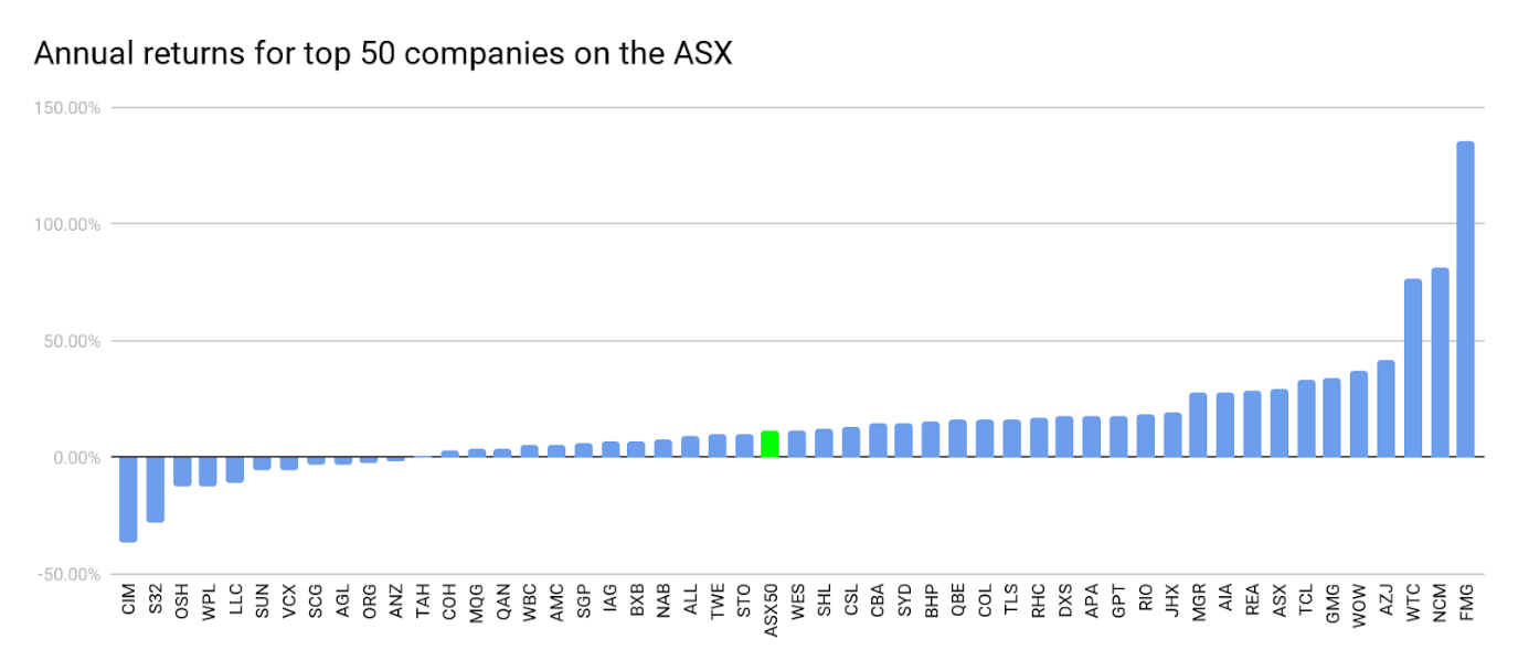
In finance, the concepts of risk and return are very much related. For now, we can think of the return on an asset, such as a stock, as the change in the asset’s value over a given time. To get a sense of how returns for different stocks may vary we have plotted the 1 year returns (September 2018 to September 2019) of the 50 largest (by market capitalisation) stocks on the Australian Securities Exchange (ASX), this is shown in Figure 1 below.
The return on the ASX50 index is also plotted as a reference[1]. As we can see, most stocks had a return that was fairly close to that of the index (around 11%), but some had returns that were much less (even negative) or much more. Looking at these companies with the benefit of hindsight, one would have done best to invest in Fortescue Metals Group Limited (FMG), the company with the highest return. Likewise, an investment in Cimic Group Limited (CIM) stock, which had the lowest return (a negative return in fact), would have turned out poorly. Based on this information, would it be wise to invest in FMG today? What about CIM?
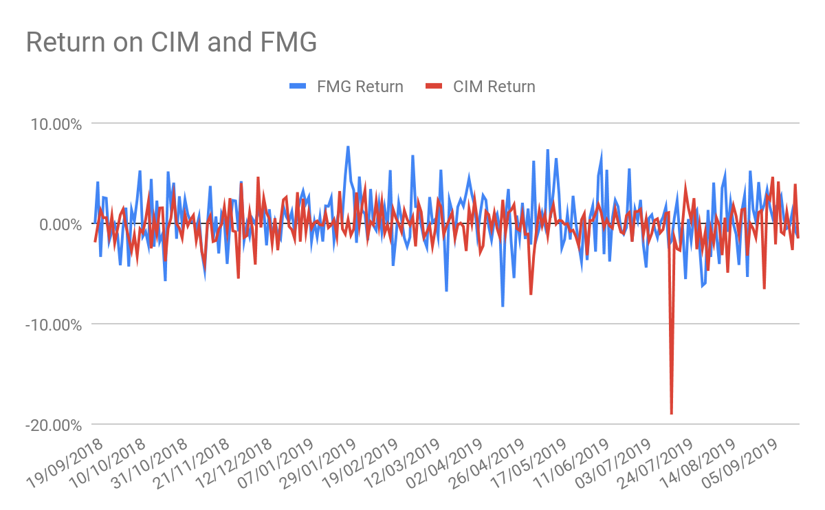
Let’s take a closer look at the two extreme cases: CIM and FMG. Figure 2 below plots the daily returns for these two stocks. Apart from a couple of outlying values, the plot of returns looks fairly similar for both companies. The average daily return for both stocks is close to 0% and rarely do the daily returns exceed plus or minus 4% for either company.
Looking at this plot we can begin to get a feel for the concept of risk.
To start with, we can think of risk on a stock as its chance to being much higher or lower than its expected value. We can take the expected value to be the mean or average value. From our discussion so far we can say that the daily returns for both FMG and CIM have an expected value of around 0%[2].
To measure how far from expectations the return might move, we can employ the standard deviation measure. The standard deviation quantifies the amount of variation in a set of values. A low standard deviation indicates that values in the set tend to be close to the mean, while a high standard deviation indicates that the values are more spread out.
It turns out that the standard deviations for FMG and CIM are 2.65% and 2.14% respectively. This means that the daily returns on FMG were more spread out over the year when compared to CIM, thus making FMG a riskier stock. With this new information, would you rather invest in FMG or CIM today?
This question is complex and we still require a few more pieces to answer it. For one, how long do you plan to hold the stock? Also, will you be investing in the stock on its own or adding it to a portfolio of assets? We will explore these questions in the following sections.
10.2.2 Holding Period and Expected Return
Previously, in Figures 1 and 2 we showed the returns on different stocks. How did we arrive at these values?
We stated earlier that the return on a stock can be thought of as the change in the stock’s value over a given time. So, let’s say you purchased a share of FMG stock in September 2018. You would have paid $3.79 per share. If you sold that stock in September 2019 you would have sold at a price of $8.92. Therefore you would have made...
[latex]\$ 8.92-\$ 3.79=\$ 5.13[/latex]
...over the year. This increase in value from buying the stock at a low price and selling at a higher price is known as the capital gain. Similarly, if you had purchased a share of CIM stock in September 2018 for $51.27 and sold in September 2019 for $31.83 you would have received a capital gain of...
[latex]\$ 31.83-\$ 51.27=-\$ 19.44[/latex]
which is a capital loss of $19.44.
A stock’s return comes not only from the capital gain or loss, but also from the dividends received. In the case of our two stocks, dividends paid between September 2018 and September 2019 were...
|
FMG |
CIM |
||
|---|---|---|---|
|
Date |
Dividend |
Date |
Dividend |
|
02 Sept 2019 |
$0.24 |
11 Sept 2019 |
$0.71 |
|
22 May 2019 |
$0.60 |
13 June 2019 |
$0.86 |
|
28 Feb 2019 |
$0.19 |
|
|
Table 1: Dividend dates and amounts for FMG and CIM stock between 09/2018 and 09/2019.
So an investor in FMG stock would have received a total of $1.03 in dividends and an investor in CIM would have received $1.57. Knowing both the capital gain/loss and dividends paid we can now compute the Total Dollar Return (TDR) for these two stocks.
[latex]\begin{array}{l}{\text { TDR = Dividend Income + Capital gain/loss }} \\ {\text { TDR }_{F M G}=\$ 1.03+\$ 5.13=\$ 6.16} \\ {\text { TDR }_{C I M}=\$ 1.57-\$ 19.44=-\$ 17.87}\end{array}[/latex]
Calculating total dollar returns gives some information about the stocks but it does not allow us to compare across stocks. For example, if two stocks offer a total dollar return of $10 but one has a price of $10 while the other has a price of $100, which would you rather invest in?
To compare across stocks, we should normalise the returns in some way. This could be done by taking holding period returns, which measures the return relative to the initial price, and is calculated as follows:
[latex]\begin{array}{l}{\text { Holding period return = Total dollar return/Price}_{\text {t-1 }}} \\ {\text {Holding period return}_{\text {FMG }} =\$ 6.16 / \$ 3.79=1.635 \text { or } 163.5 \%} \\ {\text { Holding period return}_{\text {CIM }}=-\$ 17.87 / \$ 51.27=-0.349 \text { or }-34.9 \%}\end{array}[/latex]
This holding period return is the return received from holding an asset over a certain period of time. A useful exercise would be to understand how much of the holding period return stems from the dividend and how much from the capital appreciation3.
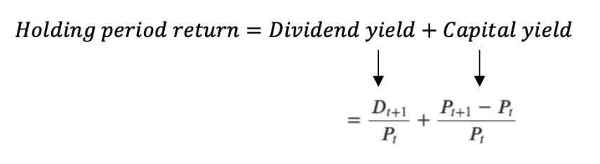
...where [latex]t[/latex] is the period the stock was purchased [latex]P[/latex] refers to the price of the stock at time [latex]t[/latex], and [latex]D[/latex] refers to the dividend. Note that this is a simplified 1-period model only.
Applying this to our stocks FMG we see that...
\begin{equation} \begin{aligned} \text { Holding Period Return}_{F M G}=\frac{D_{t+1}}{P_{t}}+\frac{P_{t+1}-P_{t}}{P_{t}} \\=& \frac{$1.03}{\$ 3.79}+\frac{\$ 8.92-\$ 3.79}{\$ 3.79} \\ &=0.272+1.354 \\ &=1.635 \text { or } 163.5 \% \end{aligned} \end{equation}
[latex]\begin{aligned} \text { Holding Period Return}_{F M G}=\frac{D_{t+1}}{P_{t}}+\frac{P_{t+1}-P_{t}}{P_{t}} \\=& \frac{$1.03}{\$ 3.79}+\frac{\$ 8.92-\$ 3.79}{\$ 3.79} \\ &=0.272+1.354 \\ &=1.635 \text { or } 163.5 \% \end{aligned}[/latex]
FMG had a holding period of 163.5% which is composed of a 135.4% capital gain yield and a 27.2% dividend yield.
Concept Check
What is the dividend yield for CIM?
Remember that CIM started the year at $51.27, ended the year at $31.83 and paid dividends totalling $1.57 per share.
What is the capital gains yield for CIM?
Remember that CIM started the year at $51.27, ended the year at $31.83 and paid dividends totalling $1.57 per share.
What is the holding period return for CIM?
What is the cause of the negative holding period return?
10.2.3 Average Returns
Another bit of information an investor might want to know is how their stock did on average during the holding period. Thus, they could calculate the mean return during the holding period:
[latex]\bar{x}=\frac{1}{t} \sum_{i=1}^{t} x_{i}=\frac{x_{1}+x_{2}+\cdots+x_{t}}{t}[/latex]
...where [latex]t[/latex] is the number of periods for which the stock was held, [latex]x_{i}[/latex] refers to the return for the [latex]i^{th}[/latex] period, and [latex]\bar{x}[/latex] is the average, or arithmetic mean. In the case of FMG and CIM, the mean daily returns (around 260 observations) during the period from September 2018 to September 2019 were...
[latex]\begin{array}{l}{\overline{\text {return}}_{F M G}=0.43 \%} \\ {\overline{\text {return}}_{C I M}=-0.15 \%}\end{array}[/latex]
So, on any given day during this period, an investor in FMG stock could have expected to receive a return of 0.43% over the previous day and an investor in CIM could have expected to receive a return of -0.15%. Of course these values are arrived at with the benefit of hindsight. An investor in September 2018 could not have known with certainty that these would be their actual returns.
10.2.4 Expected Return
The expected return is a return that can be estimated by calculating the probability-weighted average of the possible returns from an investment. The probability weights are based on information that an investor has at the time.
[latex]E\left[R_{i}\right]=\sum_{j=1}^{n} p_{j} R_{i j}=p_{1} R_{i, 1}+p_{2} R_{i, 2}+\cdots+p_{n} R_{i, n}[/latex]
where [latex]n[/latex] is the number of possible states (possible returns) [latex]R[/latex], and [latex]p_{j}[/latex] is the probability assigned to state [latex]R_{j}[/latex].
Let’s say we know the probability of different states of the economy and regulations concerning our product, and what the expected returns would be in each of these states. See estimates for the stock returns of FMG under different scenarios in the table below.
|
State (i) |
pi |
E(RFMG,i) |
|---|---|---|
|
1 - Recession & unfavourable regulation |
0.10 |
-20% |
|
2 - Recession & favourable regulation |
0.15 |
-10% |
|
3 - Normal & unfavourable regulation |
0.20 |
-5% |
|
4 - Normal & favourable regulation |
0.30 |
10% |
|
5 - Good & unfavourable regulation |
0.10 |
15% |
|
6 - Good & favourable regulation |
0.15 |
25% |
Note that the sum of all of the probabilities ([latex]p_{i}[/latex]) must be 1.00 or 100%.
Here we can see that the worst outcome of a recession combined with unfavourable regulation has a 10% probability of occurring and would result in a 20% loss. On the other hand, the most favourable scenario of a booming economy paired with favourable regulation would result in a 25% return and has a 15% chance of occurring. We can calculate the expected return as follows:
[latex]\begin{array}{l}{E\left[R_{F M G}\right]=\sum_{j=1}^{n} p_{j} R_{i, j}=p_{1} R_{F M G, 1}+p_{2} R_{F M G, 2}+p_{3} R_{F M G, 3}+p_{4} R_{F M G, 4}+p_{5} R_{F M G, 5}+p_{6} R_{F M G, 6}} \\ {E\left[R_{F M G}\right]=\sum_{j=1}^{n} p_{j} R_{i, j}=(0.1 *-0.2)+(0.15 *-0.1)+(0.2 *-0.05)+(0.3 * 0.1)+(0.1 * 0.15)+(0.15 * 0.25)} \\ {E\left[R_{F M G}\right]=0.0375 \text { or } 3.75 \%}\end{array}[/latex]
Thus, based on the estimations above, the expected return on FMG is 3.75%. Note that in reality it is very hard to estimate the probability of certain states occurring and the accompanying return if this state occurs. Therefore, we will give you this information.
Concept Check
The following table shows the probabilities of different states of the economy and corresponding expected returns for Goldio Ltd (GLD).
|
State (i) |
Pi |
RGLD,i |
|---|---|---|
|
1 - Severe Recession |
10% |
30% |
|
2 - Recession |
15% |
20% |
|
3 - Neutral |
50% |
0% |
|
4 - Mild Boom |
15% |
-10% |
|
5 - Large Boom |
10% |
-20% |
What is the expected return for Goldio Ltd?
10.3 Measuring Risk
In this video, you will see a first introduction to risk. In this section we look at how exactly we can measure risk.
Video: Relationship between risk and return (YouTube, 3m8s)
10.3.1 Introduction to Measuring Risk
10.3.1.1 A First Introduction to Risk
To understand risk we can start by making frequency distributions of the returns on our two stocks, FMG and CIM. To construct a frequency distribution from a data set first divide the data into bins of equal size that cover the range of values in the data set. Then count the number of values from the data set that fall into each bin.
There is a video at the end of this session explaining measuring risk, if you prefer to watch, you can skip ahead to the video.
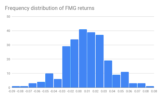
For example, in our frequency distribution of FMG daily returns (shown in Figure 3), we have created bins that are 0.01 units wide each. The bins cover the range from -0.09 to 0.08, which is sufficient to categorise the range of return values in our FMG return data set. We can see by the height of the tallest bin that there are 41 occurrences of FMG daily stock returns within the range of 0 and 0.01. This makes sense as the mean value of FMG returns is 0.0043 (0.43%). We can also see that there are very few occurrences of returns at the far ends of the range covered by the distribution. Overall, about 72% of the values lie within the range of -0.03 and 0.03.
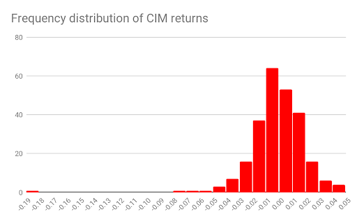
We can compare the frequency distribution of FMG returns with that of CIM (Figure 4). The tallest bin contains 63 occurrences of returns within the range -0.01 and 0.01 and, not surprisingly, the mean return on CIM is -0.0015 (-0.15%). You’ll also notice that CIM has one outlying return in the range of -0.19 and -0.18. This corresponds to what we saw in Figure 2. Apart from this extreme case, however, most of the returns, around 78%, lie within the range of -0.02 and 0.02. This means that, when compared to FMG, CIM returns exhibit smaller deviations away from their mean value.
We have already mentioned that the standard deviation (also known as the volatility4) is a measure of dispersion or risk. The standard deviation (represented by the symbol σ) of returns is calculated as follows...
4 To be precise, volatility in finance refers to the standard deviation of logarithmic returns.
[latex]\sigma=\sqrt{\frac{1}{t-1} \sum_{i=1}^{t}\left(x_{i}-\bar{x}\right)^{2}}=\sqrt{V a r}=\sqrt{\sigma^{2}}[/latex]
...where [latex]t[/latex] is the number of periods for which the stock was held, [latex]x_{i}[/latex] refers to the return for the [latex]i^{th}[/latex] period, and [latex]\bar{x}[/latex] is the mean return. The last two equalities tell us that the standard deviation is the square root of the variance ([latex]Var[/latex] or [latex]σ^{2}[/latex]). The variance measures the squared deviations from the mean. You will not be expected to compute variance from raw data in this course. The purpose of going through the computation here is to give you an idea of what factors lead to large levels of volatility or risk.
To see how to calculate the standard deviation, we can look at the monthly returns for FMG and CIM between September 2018 and September 2019. In Table 2 below we have listed the monthly stock prices for FMG and CIM during this time5. We have calculated the mean of the monthly returns and used this to calculate the deviation of each month’s return from the mean. We then take the square of these values and divided them by the number of observations (12) minus 1. Finally, we take the square of this value to arrive at the standard deviation.
5 We have taken the monthly stock price to be the price on the 1st of the month. The prices in this table have been adjusted to include dividends.
|
Date |
Price |
Return |
Deviation |
Squared Deviation |
||||
|---|---|---|---|---|---|---|---|---|
|
Month |
FMG |
CIM |
FMG |
CIM |
FMG |
CIM |
FMG |
CIM |
|
09/2018 |
$3.33 |
$49.18 |
|
|
|
|
|
|
|
10/2018 |
$3.41 |
$44.80 |
2.40% |
-8.91% |
-6.76% |
-5.69% |
0.46% |
0.32% |
|
11/2018 |
$3.56 |
$41.28 |
4.40% |
-7.86% |
-4.76% |
-4.64% |
0.23% |
0.22% |
|
12/2018 |
$3.63 |
$40.91 |
1.97% |
-0.90% |
-7.19% |
2.32% |
0.52% |
0.05% |
|
01/2019 |
$4.17 |
$42.90 |
14.88% |
4.86% |
5.72% |
8.08% |
0.33% |
0.65% |
|
02/2019 |
$5.58 |
$47.29 |
33.81% |
10.23% |
24.65% |
13.45% |
6.08% |
1.81% |
|
03/2019 |
$6.17 |
$47.77 |
10.57% |
1.02% |
1.41% |
4.23% |
0.02% |
0.18% |
|
04/2019 |
$7.01 |
$47.50 |
13.61% |
-0.57% |
4.45% |
2.65% |
0.20% |
0.07% |
|
05/2019 |
$8.35 |
$44.72 |
19.12% |
-5.85% |
9.95% |
-2.63% |
0.99% |
0.07% |
|
06/2019 |
$8.46 |
$44.39 |
1.32% |
-0.74% |
-7.84% |
2.48% |
0.62% |
0.06% |
|
07/2019 |
$8.44 |
$35.75 |
-0.24% |
-19.46% |
-9.40% |
-16.25% |
0.88% |
2.64% |
|
08/2019 |
$7.43 |
$30.71 |
-11.97% |
-14.10% |
-21.13% |
-10.88% |
4.46% |
1.18% |
|
09/2019 |
$8.92 |
$31.83 |
20.05% |
3.65% |
10.89% |
6.87% |
1.19% |
0.47% |
|
|
|
Mean |
9.16% |
-3.22% |
Standard Deviation |
9.16% |
-3.22% |
|
Table 2: Calculation of standard deviation of monthly returns for FMG and CIM stock.
Note that the standard deviation for monthly returns of CIM stock is much smaller than that of FMG stock. We do not require you to be able to calculate the standard deviation, but rather understand what the standard deviation tells us.
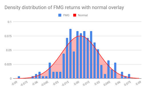
To further our understanding of frequency distributions, means, and standard deviation as a measure of risk we can compare the distributions plotted in Figures 3 and 4 to the normal distribution. The normal distribution gives the probabilities across a range that a normally distributed random variable will occur at a given point within that range. Variables are generated by selecting a mean value and standard deviation. Then the random variables will occur with highest probability at and close to the mean value and the probability of occurrence will start to decrease the farther you are from the mean. In Figure 5 we have again plotted the distribution of daily FMG returns (this time with bins that are 0.005 units wide) and overlaid this with a normal distribution that has the same mean and standard deviation as that of the FMG returns6. As you can see, the normal distribution is a good approximation for the distribution of FMG returns7. The same can be said for CIM returns.
6 Note that the FMG distribution and normal distribution have been scaled appropriately for comparison. Specifically, we have plotted the density distribution, which means that each frequency value in the given series has been divided by the sum of all frequencies in that series in order to arrive at density values. In this way, the sum of densities is equal to 1.
7 In practice, the normal distribution is used to approximate the distribution of logarithmic returns. Economists believe that stock returns are log-normally, as opposed to normally, distributed.
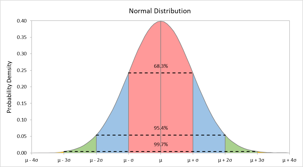
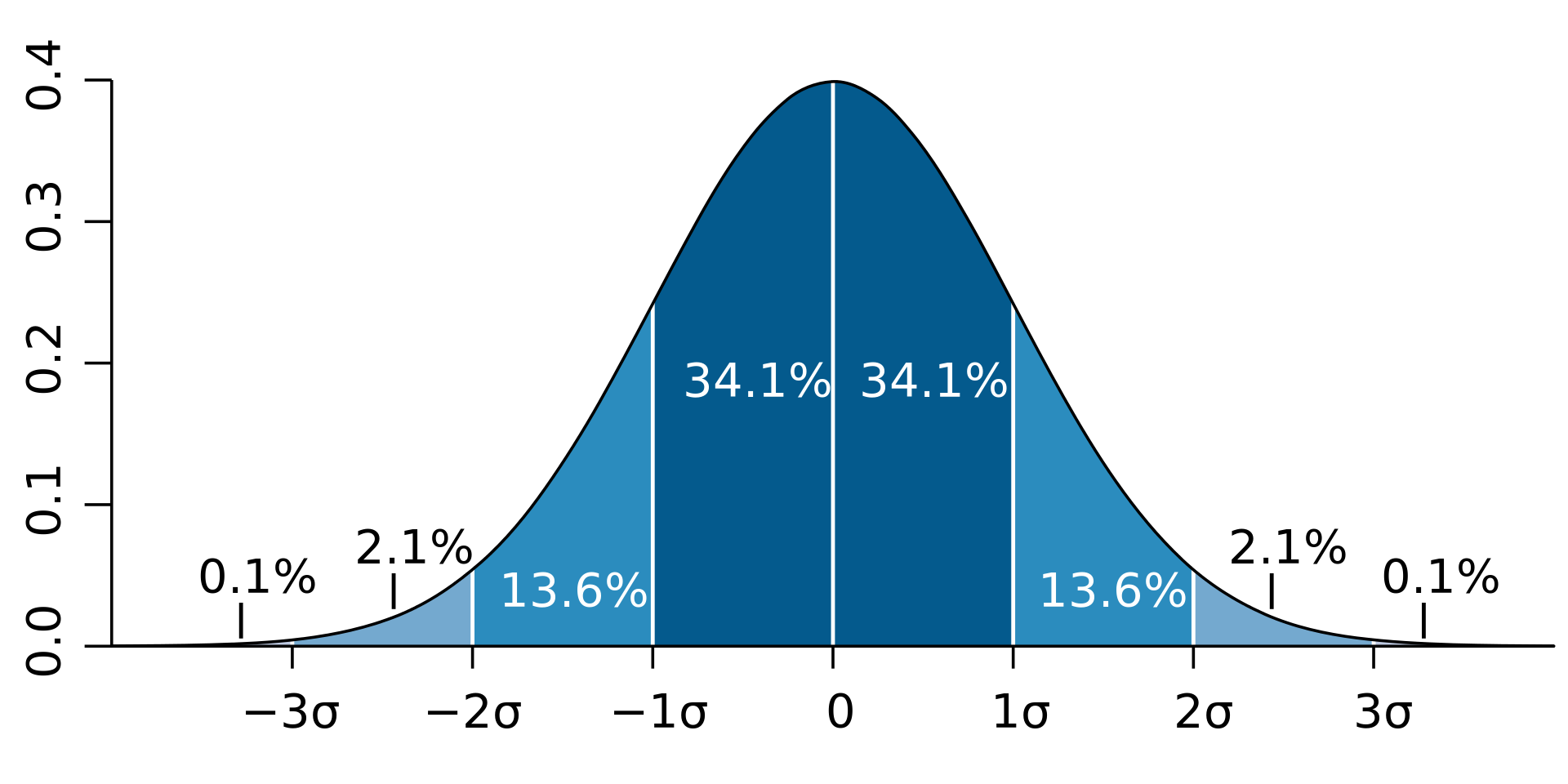
The normal distribution is useful because of its simplicity and its wide applicability. Using just the mean and standard deviation calculated from historical return data, the normal distribution allows us to approximate the probability of achieving a particular return in the future. Moreover, the more historical data you use to compute your mean and standard deviation, the better will be your approximation. If you expect your future returns are normally distributed then there is a 68% probability that you will receive a return that is within 1 standard deviation away from the mean, a 95% probability that you will receive a return that is within 2 standard deviations away from them mean, and less than 1% probability that your return will be greater (or less) than 3 standard deviations away from the mean.
For example, using FMG daily return data we have a mean of 0.43% and a standard deviation of 2.65%. If we approximate future FMG daily returns to be normally distributed with this mean and standard deviation then there is a 68% probability that the future daily return will be between -2.22% and 3.08%.
Video: Module 10 – Measuring Risk (YouTube, 14m49s)
Concept Check
Which of the following frequency distributions would be the most representative of CIM’s future daily returns?
1 point possible (ungraded)
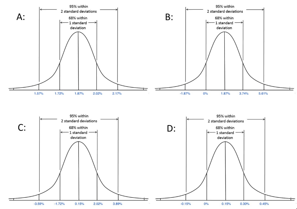
If we expect the daily mean (μ) for CIM to be 0.15% and the standard deviation (σ) to be 1.87%, and future returns to be normally distributed, which of the following frequency distributions would be the most representative of CIM’s future daily returns?
As a final visualisation, we have plotted in Figure 6 the normal distributions that were produced by using, respectively, the mean and standard deviation of daily FMG returns and that of daily CIM returns. Again, the two distributions have been scaled to allow for comparison8.
8 Note that the range of the x-axis in Figure 6 does not explicitly include the outlying negative value we saw for CIM returns in Figure 4. However, this value is accounted for in the lowest bin (-0.09 to -0.085) used here.
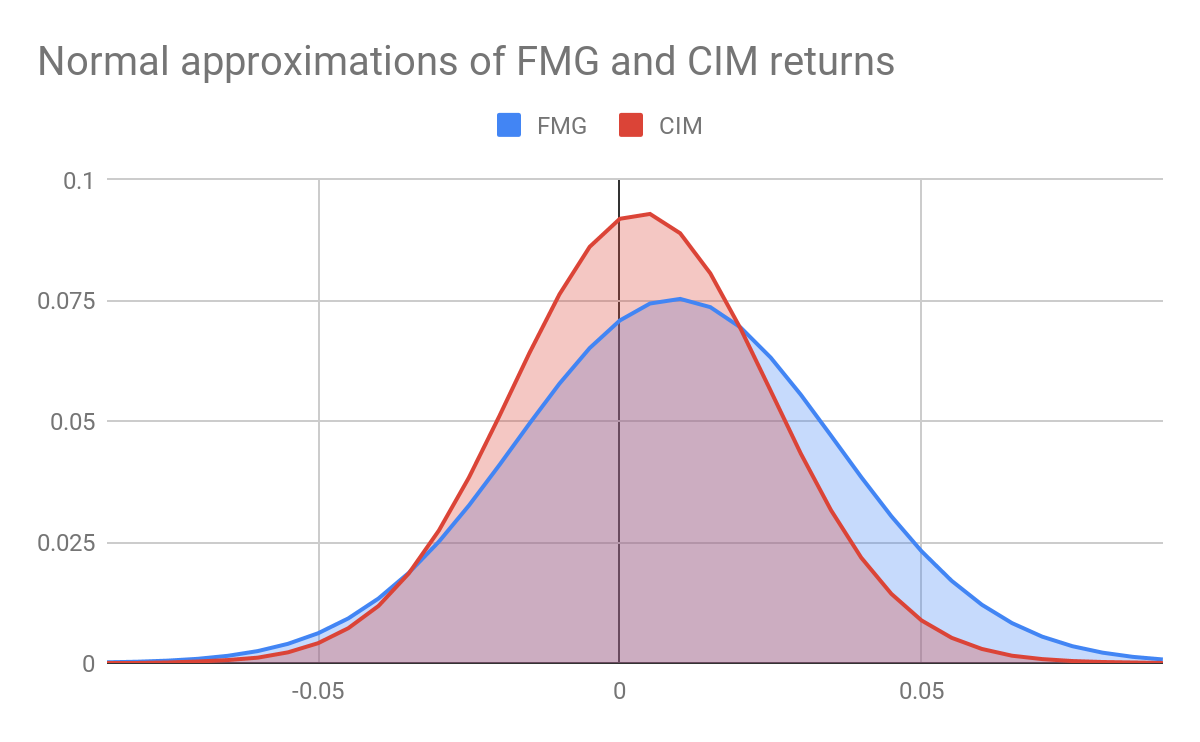
Note that the CIM normal distribution is taller and slimmer than that of FMG reflecting the fact that daily CIM returns have a smaller standard deviation. Also note the position of the peaks of the distribution. FMG stock has a higher average daily return than CIM.
Now that we have discussed both risk (as measured by the historical standard deviation) and expected return (as measured by the historical mean), we can begin to see a connection between these two quantities. Comparatively, FMG stock has the higher risk but it also has the higher expected return. The opposite is true of CIM stock, it has lower risk and lower expected return. It is often the case that a stock with a higher risk is expected to yield a higher return (otherwise no one would buy it!), however there are some risks that matter more than others; this is what we will learn in the next section.
10.4 Diversification
10.4.1 Expected Return of a Portfolio
So far we have presented the question of investing in FMG and CIM stock as mutually exclusive. That is, we have asked if an investor would rather invest in FMG or CIM stock based on the information available on past returns. However, the investment decision does not have to be an either or. Typically, investors hold portfolios of many financial assets, which can include stocks, bonds, and cash, so that their wealth is allocated amongst different assets. That is, most investors have diversified holdings.
Expected return of a portfolio
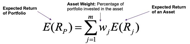
As we have mentioned, an investor who holds a portfolio of stocks allocates their wealth among the different stocks in their portfolio. Let us imagine we want to construct a portfolio from our two stock FMG and CIM. If we have $100 to spend, we could spend a certain amount, lets say [latex]x[/latex] dollars, buying FMG stock, and the rest, [latex]$100 - x[/latex], buying CIM stock. It is better to work with percentages here so we can say that we place [latex]w[/latex] percentage of our wealth on FMG stock and [latex]1-w[/latex] percentage of our wealth on CIM stock. These values [latex]w[/latex] and [latex]1-w[/latex] are called the portfolio weights. Then our expected return on the portfolio will just be the weighted average of the expected returns on the individual stocks
[latex]E\left(R_{p}\right)=w\times E\left(R_{F M G}\right)+(1-w) \times E\left(R_{C I M}\right)[/latex]
Mathematically, this is the same formula we saw in Equation 4. In fact, we can generalise for the return on a portfolio of [latex]m[/latex] assets...
Going back to our two stock portfolio, if we decide to allocate an equal amount of wealth between FMG and CIM stock we will have an expected daily portfolio return of...
[latex]\begin{aligned} E\left(R_{p}\right)=w_{F M G} & \times E\left(R_{F M G}\right)+(1-w_{F M G}) \times E\left(R_{C I M}\right) \\ &=0.5 \times 0.0043+0.5 \times(-0.0015) \\ &=0.0014 \text { or } 0.14 \% \end{aligned}[/latex]
Thus, the expected daily return is 0.14%.
Video: Portfolio Return (YouTube, 1m13s)
Portfolio weights are calculated using market values, and are expressed as a percentage of the total portfolio value: if you invest $10,000 in BHP and $30,000 in CBA (and nothing else), your portfolio value is $40,000 and the weight in BHP is 10,000/40,000 = 0.25 and the weight in CBA is 30,000/40,000 = 0.75 (or 1 - 0.25).
Example – GoSun
You hold a portfolio that consists of 500 shares in GoSun worth $5 each and 300 shares in Enova worth $32 each. What are the portfolio weights of GoSun and Enova? If the expected return on GoSun is 10% and Enova is 6%, what is the expected return of your portfolio?
Download the working for the video below (PDF, 960KB).
Concept Check (Advanced)
Your friend Jay decided to invest part of his Christmas bonus. He is a big fan of Apple and Tesla, and decides to invest in these two companies. The share prices, amounts bought, and expected return for each on the day he bought the shares are displayed below (Share prices are at 31 Oct 2019, expected returns are based on a 5 year historical average).
|
Company |
Share Price |
Number of Shares |
E(R) |
|---|---|---|---|
|
Apple |
$243.26 |
20 |
21% |
|
Tesla |
$315.01 |
25 |
9% |
1a) What are the portfolio weights for Apple in Jay’s portfolio at the day he purchased the shares?
1b) What are the portfolio weights for Tesla in Jay’s portfolio at the day he purchased the shares?
2) What is the expected return of the portfolio?
10.4.2 Portfolio Risk
Just based on the expected return, the advantage of holding a portfolio of the two or three stocks as opposed to just investing in one stock is unclear. To understand the advantage we must look at portfolio risk.
Portfolio risk depends on three items:
- Portfolio weights
- Risk (standard deviation) of the individual assets
- The relationship (correlation) between the assets
As you can see, the risk on a portfolio of stocks is not simply the weighted average of the risks of the individual assets. In fact, portfolio risk is less than the weighted average of the risks of the securities in the portfolio, and how much less depends on how strong the relationship is between the returns on the securities in the portfolio. The strength of a relationship between two variables can be measured by calculating the correlation coefficient. Correlation measures how much two random variables tend to move in the same direction or in opposite directions - it is a standardised measure and varies between -1 and +1 for all pairs of random variables, where;
- Correlation of +1 means the two variables always move in the same direction (also called perfectly positively correlated)
- Correlation of -1 means the two variables always move in opposite directions (also called (perfectly negatively correlated)
- Correlation of 0 means there is no relationship between the two random variables
Whenever we add assets to our portfolio that have a correlation of less than 1 to the assets in our portfolio something magical happens; the risk of the portfolio is less than the weighted average of the risk of the individual assets. In other words, some of the variation of the portfolio disappears!
This magical effect is what we call the portfolio effect.
Let’s have a look at how this works.
It turns out that the correlation between daily FMG and CIM returns is 0.1084 (for calculations see the Appendix) meaning that the returns on the two stocks are slightly positively correlated. A possible reason for this weak correlation is that the two companies are in somewhat different businesses. CIM is large project developer which is involved in the telecommunications, engineering and infrastructure, building and property, mining and resources, and environmental services industries. FMG, on the other hand, concentrates on the mining, processing, and transportation of iron ore.
The weak correlation between the two stocks will allow us to create a diversified portfolio with a lower combined risk than that of the individual stocks. Generally, the weaker the correlation between the two stocks the greater the risk-lowering effect of diversification.
Why does lower correlation lead to lower risk in a portfolio?
Very roughly, you can think of correlation as the probability that the two stocks will move in the same direction. If you own two stocks that always move in the opposite direction (correlation is close to -1), then when one stock goes up, the other is likely to go down. This means that gains in one stock offset the losses in the other stock. When you add the returns of the two stocks together, they offset each other and are likely to be very near the average return. In other words, the risk or variability of your return will be low. On the other hand, if your two stocks have correlation close to +1, then they will, on average, move in the same direction. On a good day, both will go up and you’ll have a very good return. On a bad day, however, both will go down and you’ll have a very bad return. So, the closer the correlation is to +1, the closer the risk of your portfolio will be to the average risk of your two stocks. And as the correlation moves towards -1, the risk of the portfolio reduces to something that is much less than the average risk of your two stocks.
To see how this works, let us take our 50/50 portfolio in FMG and CIM. In the previous section, we already took step 1 of calculating portfolio expected return (daily):
For calculating portfolio risk, we need the portfolio weights (0.5 each), individual asset risk (FMG = 2.65% and CIM = 2.41%), and the correlation (0.1084). The resulting portfolio risk (see Appendix 2 for calculations) is 0.0179 or 1.79%.
This standard deviation of the daily returns on the portfolio with equal weights given to FMG and CIM stocks is significantly less than that of either stock separately. Taken together with the return calculated above, it might be that a risk averse investor prefers investing in this lower risk portfolio over an investment in solely the higher return, but higher risk, FMG stock.
Of course, our imaginary investor is not restricted to allocating equal amounts of their wealth to FMG and CIM. They could place different weights on these two stocks in their portfolio to arrive at a risk return profile that suits their needs. This is illustrated in Figure 7 below.
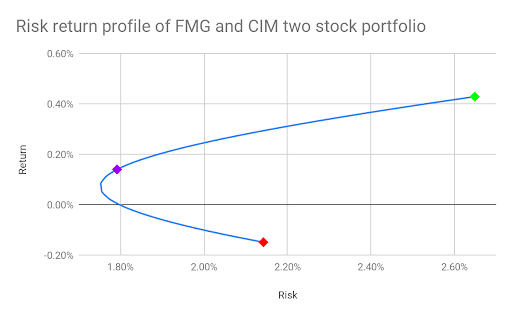
This plot is the result of calculating the portfolio mean (return) and standard deviation (risk) for different combinations of weights placed on the two stocks FMG and CIM. For any particular combination, the weights, given as percentages of the investor’s wealth, have to add to 1. For example, the investor may place 70% of their wealth in FMG and 30% in CIM, resulting in a portfolio return of 0.26% and risk of 2.03%. Note that the “portfolio” of investing in just FMG and that of just investing in CIM are also plotted. It seems from the plot that if an investor seeks the least risky portfolio of FMG and CIM stock, they should place 40% of their wealth in FMG and 60% in CIM. This portfolio will deliver a positive expected return (although lower than that of just investing in FMG stock) but also benefit from the lower risk of CIM stock.
Concept Check
Which component impacts portfolio risk but not portfolio return?
10.5 Systematic and Unsystematic Risk
In the previous section we found that portfolio risk reduces when we combine stocks with correlations that are less than perfectly correlated. How can this happen?
Video: Risk Diversification (YouTube, 3m18s)
As the video shows, there are two types of risk that are important to distinguish between.
First, let’s take a step back. The risk from owning a stock comes from unexpected changes in the value of the stock. Therefore, we could think of the actual return received from holding a stock as having two components: the expected return and the unexpected return.
We have already spoken about the expected return component. The unexpected component comes from the fact that stocks are risky and this riskiness can result in unexpected changes in the value of the stock. These changes might be due to, for example, the central bank of a country unexpectedly increasing or decreasing the interest rate. They may also be due to the government releasing unexpected news about the country’s GDP or inflation rate. You might imagine that these types of changes/announcements would affect all the companies that operate in that country. Take inflation: an unanticipated increase would likely affect wages and both the cost of goods that companies buy (accounts payable) and sell (accounts receivable).
There are other types of changes/announcements that would affect certain companies more than others. For example, the government might announce the imposition of tariffs on goods from a certain industry, or new regulations regarding certain environmental factors (e.g. the use of a waterway or limits on a particular source of pollution). Non-governmental action may also affect companies such as workers from a certain industry deciding to unionise or the discovery of new precious metal deposits. You could imagine that the discovery of a new iron ore deposit in Australia would affect FMG’s value more so than CIM’s. And some of these announcements may affect one company alone. The worst daily return for CIM came on the day that it announced its half-year earnings. Clearly, the market did not expect the reported 15% drop in profit.
What we are describing here is the difference between systematic and unsystematic risk. It is important to distinguish between these two sources of risk as an investor can themselves deal with one but not the other by using the diversification principle behind portfolio building. We will see also that this ability for an individual investor to diversify is also recognised by the market and thus affects the return that the investor expects to receive. For now, let us rewrite Equation 10 to account for these two components of unexpected returns...
So the total return on a particular company’s stock includes the expected return, some unexpected return that is due to risk factors which affect the market as a whole, and some unexpected return that is due to risk factors that are more or less unique to the particular company9.
9 The distinction between systematic and unsystematic risk may be less than exact in practice. This is because of the interconnectedness of the market. Even the most particular piece of information about a specific company can have some small effect on the market as a whole.
Concept Check
Choose if the events are systematic or unsystematic risk:
10.5.1 Systematic and Unsystematic Risk in a Portfolio
As we have seen, by building a portfolio of stocks an investor can decrease their overall risk, particularly if the returns of the stocks in the portfolio are weakly correlated.
But, what type of risk is being reduced through diversification?
If we own a diversified portfolio, systematic risks will affect all of the companies in our portfolio to some extent, because systematic risks are those that affect the economy as a whole. Unsystematic risks, however, affect only a small number of companies in the economy. So in a diversified portfolio, these unsystematic risks would tend to cancel out. This means that the risk reduced through diversification is unsystematic.
For example, if we invest solely in FMG stock, we face the risk that our returns will decrease due to some negative shocks related to iron ore. We can reduce this risk by combining our investment in FMG with an investment in CIM, a company that is not as susceptible to risk factors due to iron ore. Of course, there will still be systematic risk factors that affect both companies. These risk factors can not be diversified away. What can be done is to eliminate as much unsystematic (or diversifiable) risk as possible by optimally diversifying your portfolio. This is illustrated in Figure 8 below.
We have plotted the total portfolio risk (as measured by the average standard deviation) for equally-weighted portfolios containing different numbers of stocks10. Notice the sharp reduction in unsystematic (diversifiable) risk that occurs with just a slight increase in the number of stocks in the portfolio. As the number of stocks increase the diversifiable risk will decrease so that the total risk (the sum of the unsystematic and systematic components) approaches the systematic risk only.
10For each portfolio of n number of stocks, a 100 sample portfolios are generated by selecting n stocks randomly from the top 50 stocks in the ASX200. From these 100 samples, an average standard deviation is computed.
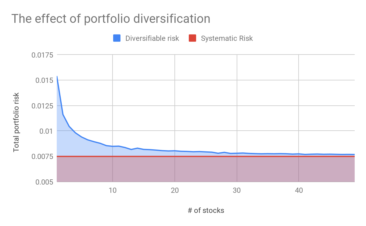
Figure 8 may be a bit misleading. It suggests that all stocks have the same level of systematic risk. This is not exactly true. While all stocks are affected by systematic risk, some are affected more so than others. Changes to the inflation rate is certainly a systematic risk but some companies might be more susceptible to these changes than others. What Figure 8 shows as the systematic risk level is really an average level (the level of systematic risk an average company will have).
So this discussion has revealed two important points:
- unsystematic risk may be reduced through diversification so that large portfolios have almost no unsystematic risk.
- different stocks are affected by systematic risk in different ways.
This leads to the systematic risk principle. The principle states that the expected return on a risky asset (such as a stock) depends only on that asset’s systematic risk. In other words, because every individual investor has the ability to diversify their portfolio in such a way as to virtually eliminate unsystematic risk, the market will only reward the investor for the risk that they can not diversify away, i.e. systematic risk.
10.6 The Capital Asset Pricing Model
In the previous sections we explored the relationship between risk and return and discovered that an asset’s expected return is determined by the systematic component of risk. Next we will quantify this systematic component and learn how we can use this to calculate a stock’s expected return.
To begin we should first discuss the concept of the risk-free asset. As we have seen in previous lessons, the price of an asset may be calculated as the present value of future cash flows. Because future cash flows are risky, we discount them with some appropriate rate of return. The more risk we assign to the future cash flows, the higher the discount rate used. Now, if an asset were truly risk-free, what discount rate would we use? Would it be zero? In other words, if you invest $100 in the asset today, would we expect to receive $100 in the future?
So that there would be no discount (there would be a 0% rate of return)?
NO!
This is not what happens in practice.
We know that there is a time value of money and therefore there should be some minimal strictly positive discount rate. In finance, when we talk about a risk-free asset we do not mean that there is absolutely no risk. Instead, we mean the tradeable asset that has the least amount of risk. In practice, this is the government bond. We have seen that government bonds do have some rate of return, albeit low.
The return on this risk-free bond (also known as the risk-free rate) may be used as a benchmark to compare the return on risky assets. The return earned on a risky asset that is above that earned on the government bond is known as the excess return.
The principle of diversification discussed earlier tells us that the market will only reward an investor for the systematic risk they take on. The unsystematic risk borne by an investor is reduced as the number of stocks in their portfolio increases. If the portfolio contains a sufficient number of stocks, the unsystematic risk is virtually eliminated. We could imagine that a portfolio that contains all the tradable assets on the market would only be subject to systematic risk. Therefore the return on this portfolio would depend only on systematic risk. While it might be difficult to construct a portfolio that contains all tradable assets (including not only stocks, bonds, and options, but also real estate, collectibles, and precious metals), we can approximate such a portfolio using market indices such as the ASX20011.
We now have the basic components to measure the systematic risk of a stock and thus its expected return. Essentially we want to compare how the excess return on the stock changes with the excess return on the market index, which contains only systematic risk. To do this we can run a simple linear regression on historical data. Linear regression is a statistical technique that fits a line to a scatter plot of data. In this case, we’re plotting the excess return of the market (measured as index return less the risk free rate) against the excess return of a single stock (measured as the stock’s return less the risk-free rate). We’re subtracting the risk-free rate in both cases because we want to measure only that portion of the return that relates to the risk of the asset.
The slope of the regression measures how the return on the stock is affected by systematic risk and is called the stock’s beta (β). A stock with a beta value of 1 is affected by systematic risk in the same way as is the market. By definition, the average stock on the market will have a beta of 1. Lower values of beta indicate the stock is less affected by systematic risk than the average stock on the market. Beta values greater than 1 indicate that systematic risk has a greater effect on that stock.
11 The ASX200 is an index portfolio comprising of stocks from the top 200 companies listed on the ASX. Each stock is weighted according to its market capitalisation (= share price x shares outstanding). Together, these 200 companies account for about 82% of the total market capitalisation on the ASX. The ASX200 is widely used as a benchmark for the Australian market.
Video: Risk Premium Systematic Risk Beta (Youtube, 3m47s)
10.6.1 Using CAPM
The expected return of a risky asset consists of the return on the risk-free asset, plus the excess return determined by the asset’s exposure to market risk.
[latex]E[r]=r_{f}+\text { excess return }[/latex]
The excess return is determined by how much systematic risk an asset is exposed ([latex]beta[/latex]) and the compensation per unit of systematic risk. Given the market has a [latex]beta[/latex] of 1, the market’s return also determines the compensation per unit of systematic risk. Therefore, we can estimate the expected return of an asset as follows:
[latex]E[r]=r_{f}+\beta\left(E\left[r_{m}\right]-r_{f}\right)[/latex]
...where [latex]E[r][/latex] is the expected return on the stock, [latex]r_{f}[/latex] is the risk-free rate, [latex]E[r_{m}][/latex] is the expected return on the market index. The quantity [latex]E[r_{m}]-r_{f}[/latex] is called the market risk premium, it’s the “premium” or excess return you earn from taking on the risk inherent in the market as a whole. This important equation is known as the Capital Asset Pricing Model or CAPM. It tells us that if we know the expected return on the market, the risk-free rate (i.e. the current yield on a government bond), and the stock’s expected beta, we can calculate an expected value for the stock’s return.
Video: Capital asset pricing model (YouTube, 3m6s)
Concept Check
If the risk-free rate for 10-year Australian government bonds is estimated to be 0.95%, the expected return on the ASX200 8.74%, and the beta for CIM is 1.40, what is the expected return for CIM?
10.6.2 Does CAPM Work?
You may find that the actual return is much higher or lower than what is predicted by CAPM. However, this does not suggest that the CAPM is a poor model in general.
The first thing to realise is that the CAPM is a forward looking model. It tells us the future return that an investor might expect on a risky investment (e.g. an investment in stock) given the fact that the market is only willing to reward the investor for taking on systematic risk. The investor may end up realising a much greater or lower return, and this will likely be the case for investments in stocks with a large amount of total risk. However, there is no way to know beforehand that these abnormal returns will indeed occur, and certainly the market will not reward the investor preemptively for them. Therefore, the CAPM is really giving us a best guess at the expected return on a stock given all the information (e.g. historical data) we have at the time of investment.
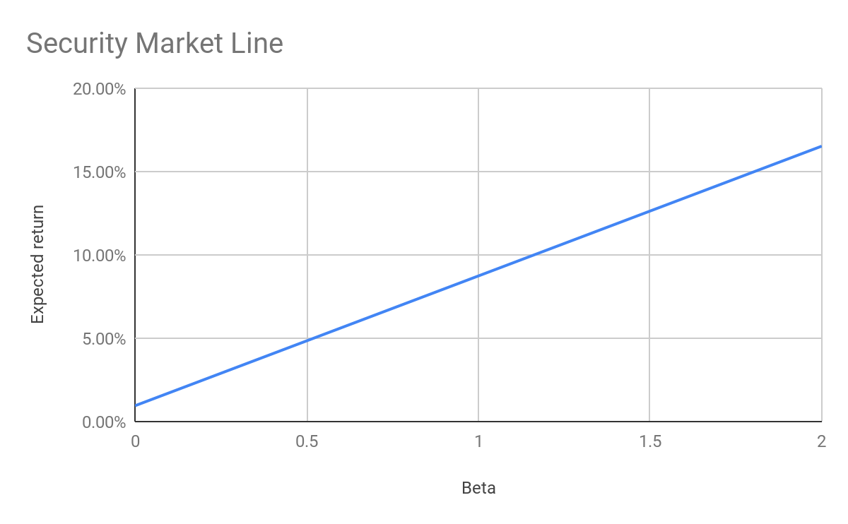
The CAPM does this by using the beta, typically estimated using the stock’s historical systematic risk vis-à-vis the market. The CAPM thus quantifies the relationship between risk and return: the larger the effect of systematic risk on a stock, the larger the return an investor expects to receive on that stock. We can visualise the CAPM’s risk return relationship using the Security Market Line (SML). In Figure 9 we have plotted the SML for the expected annual returns on ASX200 stocks with different betas12.
12 Here we have annualised daily returns calculated using the CAPM. The daily CAPM returns were calculated in turn using betas generated from historical daily return data.
10.7 Summary and Key Formulas
10.7.1 Summary
In this chapter we have covered different concepts related to both risk and return.
Hopefully you are now able to:
- Explain the relationship between risk and return
- Distinguish between, and calculate, holding period return and expected return
- Explain why standard deviation of returns is especially useful in finance (risk measure)
- Explain the concept of diversification
- Distinguish between systematic and unsystematic risk
- Explain the Capital Asset Pricing Model (CAPM)
- Evaluate the adequacy of expected return using CAPM
- Critically evaluate CAPM
which were the learning objectives outlined at the start of the chapter. See if you can write down a short paragraph on each of these questions. If you struggle, revise the chapter again and/or contact your tutor to book a consultation.
10.7.2 Key Formulas
Calculating Holding Period Return:
[latex]Holding \, Period \, Return = Dividend \,Yield\, + \,Capital\, Yield[/latex]
[latex]Holding \, Period \, Return = \frac{D_{t+1}}{P_{t}}+\frac{P_{t+1}-P_{t}}{P_{t}}[/latex]
Note: you need to be able to calculate portfolio weights, there is no formula for this in the chapter but it is explained.
- The ASX 50 is an index that represents the large-cap component of the Australian stock market. It contains the ASX top 50 companies by way of float-adjusted market capitalisation and accounts for 63% (March 2019) of the Australian equity market. https://www.marketindex.com.au/asx50 ↵
- We will see later that the historical means, or expected values, of FMG and CIM daily returns are not exactly 0. For our purposes here we can assume that the means are relatively close to 0. ↵
