6.1 Introduction

When a company wants to take on a new investment opportunity, they will often need to look for external sources of capital. We saw last week that one way for a company to do this is to take out a loan or issue a bond (debt). Another way is for that company to issue shares. Investors may agree to purchase a company’s shares because they expect that holding those shares will allow them to make claims on the future cash flows of the company. These potential shareholders will be willing to pay a price for the shares that is based on both the information that they have about the company (and thus its expected value), and the level of risk they are willing to take (how much uncertainty around the expected future values they are willing to accept).

In a large stock market, many investors, each having different beliefs and preferences around risk, will come together and trade shares. They might buy shares that are being offered or sell shares that they hold. As more and more market participants come together to trade on a particular share, a clearer picture of the “true” value of the share emerges. We can see how this works by looking at a typical day of trading on the stock market. The figure below shows the prices at which market participants were willing to buy (the bid price) and willing to sell (the ask price) shares in Tesla Motors on 20/09/2019. The figure also shows the amounts of shares investors were willing to buy (the bid volume) and willing to sell (the ask volume) at the given prices at the given times.

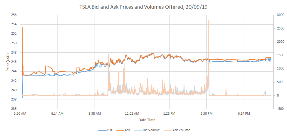The main thing to notice about this plot of stock prices is how the discrepancy between bid and ask prices decreases as the amount of trading increases. This makes sense as more trading implies that more investors are sharing their information (beliefs and preferences) with the market (through the price they offer to buy or sell at) and market participants are better positioned to arrive at a consensus value for Tesla’s share price.

In this chapter, we will look at some particular models that individual investors might use to estimate a share price that takes into account their beliefs and preferences.

6.1.1 Where Do Prices Come From?

We saw in the previous topic, Valuing Debt, that when a company requires financing, they may look to their residual cash flows (internal financing), or may seek to raise capital by issuing debt or equity. We also learned what determines the value of debt and how this may be calculated. In this lesson we will answer similar questions about equity: what determines equity value and how can share prices be calculated?

So, where do share prices come from? To answer this we could begin by recalling the determinants of the bond price: the face value and coupon payments (i.e. promised cash flow), the time to maturity, and the interest rate required by the market. For the bond, the values for these determinants of the price are easily obtained. This is not the case for shares. Shares do not necessarily have promised cash flows as it is not compulsory for companies to pay dividends, there is no set maturity date, and due to the high degree of volatility, market required returns (risk-adjusted interest rates) are difficult to observe.

Nevertheless, the present value of a share’s cash flows, and thus its price, can be estimated. Investors would have an expectation about the dividend payments they will receive from owning a share, and these dividend payments, like coupon payments for bonds, could occur at regular intervals. So we may be able to get around our first difficulty in valuing shares. What about the maturity date and the discount rate? We will see that assumptions can be made about these determinants as well.

Have a look at this Netflix video: The stock market has been booming. That doesn’t mean the economy is too. This explains what the stock market is actually measuring.

6.2 General Dividend Valuation Model

Let’s imagine that you buy a share today and have an expectation that you will be able to sell this share in one year for $9. You also expect that you will receive a dividend of $1 at the end of the year, just before you sell your share. Finally, suppose that, as an investor, you require a rate of return of 10%. What is the most you would pay for this share? Well, the most you would be willing to pay would have to be equal to the present value of the cash flows you expect to receive discounted at your required rate of return (to account for your opportunity cost!), that is

[latex]\text {Present Value}=\frac{(\mathrm{$} 1+\$ 9)}{(1+0.1)^{1}}=\$ 9.09[/latex]

Thus, if you require a 10% return on your investment, you would be willing to pay $9.09 now for receiving $9 + $1 in one year. We can generalise the formula used above as follows:

[latex]P_{0}=\frac{D_{1}+P_{1}}{(1+r)^{1}}\tag{1}[/latex]

where [latex]P_0[/latex] is the price of the share today, [latex]D_1[/latex] and [latex]P_1[/latex] are, respectively, the dividend paid and the price of the share in one year from now, and [latex]r[/latex] is the rate of return. Now, you might be saying that what we have done so far does not really help us to answer the general question of how to determine share prices. In our example we have essentially replaced the problem of determining the price of the share today with that of determining the price of the share in the next period (and we assumed what the latter would be!). But determining the price of the share in the next period is at least as difficult as determining the price today.  So how can we proceed?

Using our general formula (1) we can say that if we know the share price in period 2, then we can figure out the share price in period 1

[latex]P_{1}=\frac{D_{2}+P_{2}}{(1+r)^{1}}[/latex]

Plugging this into equation (1) we have:

[latex]\begin{aligned} P_{0} &=\frac{D_{1}}{(1+r)^{1}}+\frac{P_{1}}{(1+r)^{1}} \\ &=\frac{D_{1}}{(1+r)^{1}}+\frac{D_{2}+P_{2}}{(1+r)^{1}} \times \frac{1}{(1+r)^{1}} \\ &=\frac{D_{1}}{(1+r)^{1}}+\frac{D_{2}+P_{2}}{(1+r)^{2}} \\ &=\frac{D_{1}}{(1+r)^{1}}+\frac{D_{2}}{(1+r)^{2}}+\frac{P_{2}}{(1+r)^{2}} \end{aligned}[/latex]

But what if we do not know the share price in period 2. Well we could calculate the price in period 2 if we knew the price in period 3, and we could calculate this latter if we knew the price in period 4, etc. You might begin to recognise a pattern. We can replace the problem of knowing the share price today with one of knowing the share price sometime in the future. If we put the expected cash flows on a timeline, it would look like this:

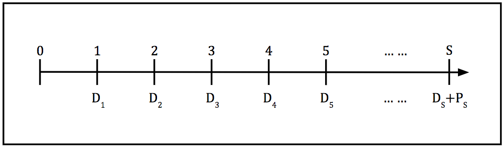
Therefore we can estimate the price of a share today using the following formula:

[latex]P_{0}=\frac{D_{1}}{(1+r)^{1}}+\frac{D_{2}}{(1+r)^{2}}+\frac{D_{3}}{(1+r)^{3}}+\frac{D_{4}}{(1+r)^{4}}+\frac{D_{5}}{(1+r)^{5}}+\ldots+\frac{D_{S}+P_{S}}{(1+r)^{S}}[/latex]

Equation (2) is often referred to as the General Dividend Discount Model. The subscript [latex]S[/latex] in the last term refers to the last period for which we make estimates of the future dividend and share price. We could imagine that period [latex]S[/latex] refers to the point at which the shareholder expects to sell their share (and realise a capital gain). However, we should not make the mistake in thinking that the share price today, [latex]P_0[/latex], is affected by the shareholders’ expectations regarding when they will sell. The share price estimated by the General Dividend Discount Model is not affected by the choice of [latex]S[/latex].  In other words, the period in which the investor expects to sell is arbitrary. The investor could sell in the next period or in 10 years (or perhaps never sell). Regardless, when they do sell, the share will likely still be valuable ([latex]P_S[/latex]) and that value may be estimated by the future cash flows (dividend payments) as well. To understand this, think about how the purchaser at time [latex]S[/latex] will value the share.

So how many dividend payments will we need to determine? Theoretically, there could be an infinite number. Obviously this would render Equation (2) practically useless. Even if the number of dividend payments is finite, how do we determine what they will be? Can we make any inferences based on our expectations? As we will see, we can make assumptions about the pattern in dividend payments that make the General Dividend Discount Model easier to use and allow us to more readily estimate the share price.

6.3 Assumptions

6.3.1 Constant Dividend Model

The General Dividend Discount Model may be simplified by making assumptions regarding the pattern in dividend payments. These assumptions will allow us to make use of formulas that we have already encountered in our discussion of Present Value methods.

The case of zero growth should be familiar. If dividend payments do not grow over time, they will remain fixed. We can visualise this on a timeline:

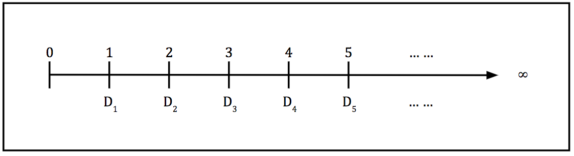
Note that all dividends are the same amount, so no subscripts (indicating time t) are needed. The price of a share with constant dividend payments will be given by:

[latex]\begin{aligned} P_{0}=\frac{D}{(1+r)^{1}}+\frac{D}{(1+r)^{2}}+\frac{D}{(1+r)^{3}}+\frac{D}{(1+r)^{4}}+\frac{D}{(1+r)^{5}}+\ldots \infty \end{aligned}[/latex]

This may be simplified. We have already seen how to calculate the present value of periodic fixed cash flows paid out in perpetuity:  the perpetuity formula. If we apply this to the case of perpetual dividend payments we have

[latex]P_{0}=\frac{D}{r} \tag{3}[/latex]

Where, D is the constant dividend, and r the require rate of return. Why is the value of something that pays an infinite number of payments not infinite? Remember that the further away a cash flow occurs, the less it is worth today because there are many years your money could earn interest over. For example, if I promise you $3 in 50 (100) years, and you require a return of 5%, you would be willing to pay me only $0.26 ($0.023) now. As our time horizon moves towards infinity, the present value moves towards zero and the infinite sum converges to a finite number.

6.3.2 Constant Growth Model

If a company is growing and we expect it to continue to do so, we may want to assume that dividends also keep growing for the foreseeable future. To keep it simple, we often assume that dividends grow at a certain fixed rate g. Using this assumption, we can estimate the value of future dividends using past dividends. For example, if [latex]D_0[/latex], the dividend in period 0 (i.e. the dividend that has just been paid), is expected to grow at the rate [latex]g[/latex], we could easily calculate the value of [latex]D_1[/latex], the dividend in period 1:

[latex]D_{1}=D_{0} \times(1+g)[/latex]

Similarly, the dividend in period 2 would be:

[latex]D_{2}=D_{1} \times(1+g)=\left[D_{0} \times(1+g)\right] \times(1+g)=D_{0} \times(1+g)^{2}[/latex]

We can generalise the above as follows (equation (4)):

[latex]D_{t}=D_{0} \times(1+g)^{t} \tag{4}[/latex]

The pattern of dividends will be:

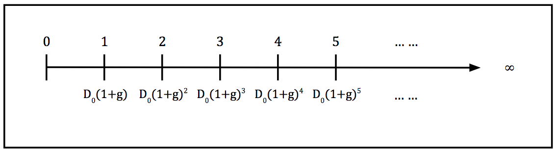
The assumption of constant growth in dividend payments allows us to simplify our share price calculation. Instead of having to determine the dividends paid in each period (as in Equation 2), we only have to know the value of the dividend that has just been paid and the growth rate. We can write out the price of the share explicitly:

[latex]\begin{aligned} P_{0} &=\frac{D_{1}}{(1+r)^{1}}+\frac{D_{2}}{(1+r)^{2}}+\frac{D_{3}}{(1+r)^{3}}+\frac{D_{4}}{(1+r)^{4}}+\frac{D_{5}}{(1+r)^{5}}+\ldots \\ &=\frac{D_{0}(1+g)^{1}}{(1+r)^{1}}+\frac{D_{0}(1+g)^{2}}{(1+r)^{2}}+\frac{D_{0}(1+g)^{3}}{(1+r)^{3}}+\frac{D_{0}(1+g)^{4}}{(1+r)^{4}}+\frac{D_{0}(1+g)^{5}}{(1+r)^{5}}+\ldots \end{aligned}[/latex]

As long as the growth rate is less than the rate of return (and the rate of return is positive) we can write the present value of this series of cash flows as

[latex]P_{0}=\frac{D_{0}(1+g)}{r-g}=\frac{D_{1}}{r-g} \tag{5}[/latex]

Equation (5) is known as the Gordon Growth Model, after the author who first published it in 1956. We may generalise this formula to find the share price in any period t.

[latex]P_{t}=\frac{D_{t}(1+g)}{r-g}=\frac{D_{t+1}}{r-g}\tag{6}[/latex]

As we will see, this generalisation is particularly helpful in situations where a company experiences non-constant or supernormal growth.

So far, we have assumed that the rate of return [latex]r[/latex] is given. This may not always be the case and certainly estimating the required return for an investor is a complex task. Nevertheless, from our discussion of the Gordon Growth Model (Equation 5) we can make some inferences about the rate of return required by the investor. Rearranging Equation (5) we have equation (7):

[latex]r=\frac{D_{1}}{P_{0}}+g \tag{7}[/latex]

This tells us that the rate required by an investor has two components:

1.  [latex]D_{1}/P_{0}[/latex], we can call the dividend yield. This is the expected cash dividend in the next period divided by the current share price.

2.  growth rate, [latex]g[/latex]. If the dividend grows at a constant rate and the required return is fixed, then the share price must grow at the same rate as the dividend. Therefore, we can call this second component of the required rate the capital gains yield. That is, the rate at which the value of the investment grows.

6.3.3 Valuation using PE Ratio

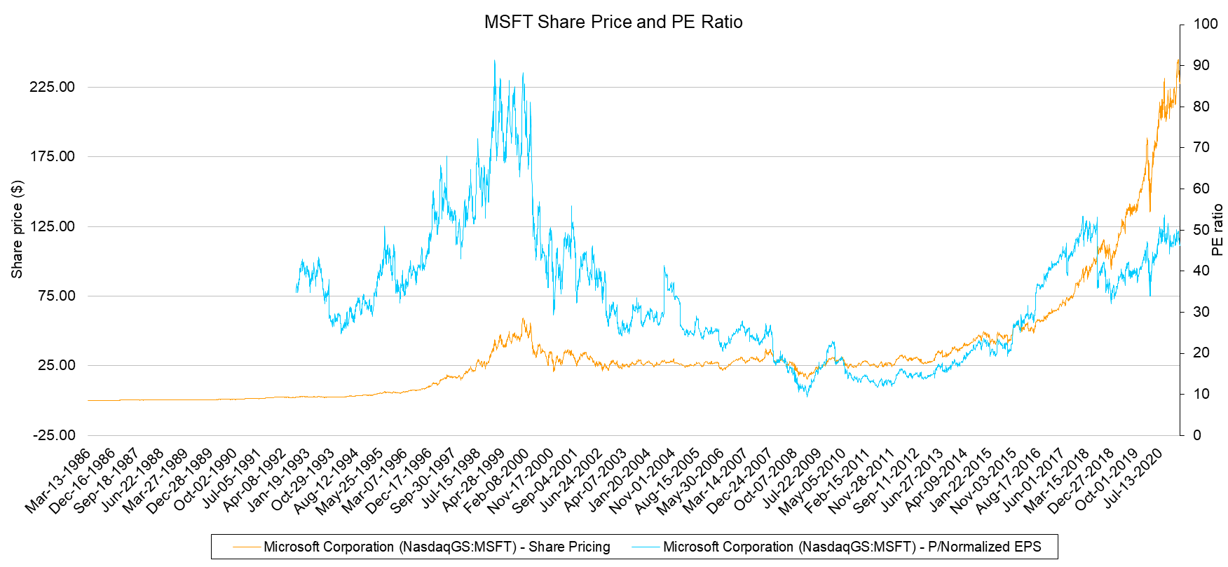
As mentioned previously, estimating the value of a share can be difficult. In the previous section, we used the General Dividend Discount model to estimate the value of a share. Due to its inherent assumptions, this method can not be readily applied to companies that do not currently pay dividends and have no intention to do so in the near future. What if the company does not pay out a dividend? Does this mean that the share price would be zero? Not necessarily. Many young firms do not pay out dividends, instead choosing to reinvest their retained earnings in profitable growth opportunities.  For example, Microsoft famously did not pay dividends for its first 17 years of operation.  Microsoft had its initial public offering in March 1986 and paid out its first dividend in January 2003.  As we can see from Figure 1 below, MSFT shares certainly had a value before dividends were paid out. More recently, Tesla has rarely made a profit since it was listed on the share market in 2010, yet its share price has increased from around $17 a share in 2010 to over $100 in 2013, then to $383 in 2017. In early 2021, the share price for Tesla has reached all-time high of over $4,500 (share split re-adjusted), with a market value over $850 billion. Importantly, Tesla has yet to pay a cent of dividend.

One way of estimating the share price for a company that does not pay out dividends is to utilise the company’s historical price earnings ratio (PE) and the current earnings per share (EPS). PE is defined as the ratio of a company’s share price to its EPS over the previous year, that is, the ratio of Price to Earnings.  Therefore, it is possible to estimate share price if we know a company’s EPS and have a benchmark PE:

[latex]P_{T}=\text { Benchmark } P E \times E P S_{t} \tag{8}[/latex]

This benchmark PE may be taken to be an average or median of current PEs from similar companies, or the average historical PE from the company whose share you want to value. Utilising benchmarks is particularly useful for estimating the share price of non-dividend paying companies, however the technique need not be limited to just these types of companies.  Benchmarking can also be used in conjunction with the General Dividend Discount Model to obtain a better share price estimate for dividend paying companies.

6.3.4 Optional Extension

The assumptions that dividend payments are either held constant or grow at a constant rate are nice but not always reasonable. We can easily allow for fluctuations in the growth rate (and even growth rates that exceed the discount rate) in the short term if we assume that the growth rate will eventually settle to a fixed value which is less than the discount rate. To see how this works, let us write out the share price explicitly

[latex]P_{0}=\frac{D_{1}}{(1+r)^{1}}+\frac{D_{2}}{(1+r)^{2}}+\ldots+\frac{D_{N}}{(1+r)^{N}}+\frac{P_{N}}{(1+r)^{N}} \tag{9}[/latex]

where [latex]P_N[/latex], the price of the share in period [latex]N[/latex], is given by:

[latex]P_{N}=\frac{D_{N}\left(1+g_{N}\right)}{r-g_{N}} \tag{10}[/latex]

and [latex]g_N[/latex] is the constant growth rate that can be applied to the dividend payments beginning in period [latex]N[/latex] (note that [latex]g_N[/latex] could be zero).

Now, we can split the task of calculating the share price in Equation (9) into two pieces:

1. Finding the present value of the dividend payments up to period [latex]N[/latex], and

2. Calculating the present value of the dividend payments that occur after (i.e. the [latex]P_N[/latex] term).  This is called the terminal value.

Obtaining the first of these two present values will be straight forward if you know all the dividend payments.  For the second part, we can use the growing perpetuity formula, to estimate the share price at year [latex]N[/latex], and then discount it back to year 0.

6.4 Calculate Share Value

Let us make use of our share price models with some examples. Consider the Nakatomi Corporation, which has been paying out dividends of $4 p.a. consistently for the past 10 years. The company’s earnings are stable and they have no plans to change their dividend policy in the foreseeable future. What might their share price be?

First, note that due to Nakatomi’s consistency with regards to earnings and dividend payout policy, investors may make the reasonable assumption that dividend payments will remain fixed in perpetuity. Therefore, we have the following timeline of cash flows.

The timeline shows that the firm has paid a constant dividend of $4 every year for the past 10 years, and that it is expected to continue to pay this dividend in perpetuity. The share price at time 0 has been calculated using the perpetuity formula, Equation 3 above. We assume that investors require a return of 5% so that

[latex]P_{0}=\frac{D}{r}=\frac{\$ 4}{0.05}=\$ 80[/latex]

(Note that this would be the price after the dividend at time 0 has been paid, otherwise it would be $80+$4=$84)

Simple enough. Now let us imagine that Nakatomi, due to some good news about their current investments, announces that they plan to pay out a dividend of $4.08 next year, $4.16 the following year, $4.24 the year after, $4.33 in four years, and so on. How might an investor value Nakatomi’s shares now?  To begin, let us draw a timeline:

It seems that Nakatomi now plans to pay an increasing dividend every year. By how much is the dividend increasing year on year?  We can calculate this easily using the dividend values in year 1 and today:

[latex]g=\frac{D_{1}-D_{0}}{D_{0}}=\frac{\$ 4.08-\mathrm{$} 4}{\mathrm{$} 4}=0.02=2 \%[/latex]

So, it seems that Nakatomi plans to increase its dividends at a steady rate of 2%. This value is consistent with the dividend payments in years 2, 3, and 4 as well. Note that this growth rate in dividends is also lower than the required rate of return, 5%. Therefore, we can use the Dividend Discount Model, Equation (5), to price Nakatomi’s share:

[latex]P_{0}=\frac{D_{0}(1+g)}{r-g}=\frac{\$ 4(1+0.02)}{0.05-0.02}=\frac{\$ 4.08}{0.03}=\$ 136[/latex]

It makes sense that the share is more valuable now if investors believe that they will receive growing dividend payments. This example also illustrates the impact of growth rate assumption on share price. Share price is very sensitive to growth rate assumption, with growth rate increases from 0% to 2% in this example, the share price could have increased by 70%.

6.4.1 Extend Your Knowledge (optional)

Now suppose that Nakatomi has received even better news about its current investments and now plans to pay a dividend of $4.4 next year, $4.84 the following year, $5.32 the year after, and then settle to the steady growth rate of 2% from their previous announcement. How much will investors be willing to pay for Nakatomi’s shares now? Let’s first draw a timeline:

The timeline shows that, as in the previous two cases, Nakatomi has paid an annual dividend of $4 for the past 10 years. It now plans to pay large dividends for the next 3 years and then settle down to dividends that grow at a small but steady rate of 2%. Clearly, the dividend payments are growing at a higher rate than 2% in years 1 through to 3. We can easily see that there are non-constant dividends in the first 3 years. Now we can use the mixed dividend growth model in Equations 7 and 8 with [latex]g_N=2%[/latex] as shown here…

[latex]\begin{aligned} P_{0} &=\frac{D_{1}}{(1+r)^{1}}+\frac{D_{2}}{(1+r)^{2}}+\ldots+\frac{D_{N}}{(1+r)^{N}}+\frac{D_{N}\left(1+g_{N}\right)}{r-g_{N}} \times \frac{1}{(1+r)^{N}} \\ &=\frac{$4.4}{(1+0.05)^{1}}+\frac{$4.84}{(1+0.05)^{2}}+\frac{$5.32}{(1+0.05)^{3}}+\frac{$5.32(1+0.02)}{0.05-0.02} \times \frac{1}{(1+0.05)^{3}} \\ &=\$ 13.18+\$ 156.37=\$ 169.55 \end{aligned}[/latex]

…which is the share price shown in the timeline. Again, the share price has increased on the expectation about the growth in dividend payments.

6.5 Critical Evaluation

The models we have discussed above allow estimation of the value of a share. These models rely on particular assumptions about the cash flows one expects to receive from holding the share. The share price estimated using the General Dividend Discount Model (Equation 2) relies, first and foremost, on the assumption that the company who issues the share makes dividend payments to their shareholders. As we saw with the early years of Microsoft, it is not necessarily the case that companies pay dividends and it is certainly not required that a company pay dividends in order for their shares to be valuable to investors. Even if a company does pay dividends, the information that investors receive about the company’s dividend policy can really only be used to estimate future dividend payments. So, the General Dividend Discount Model relies on expected values of future dividends. 

It is also worth noting that the majority of share value comes from dividends paid over the next 10 or 20 years. Consider the following chart. We have taken the present value of expected dividend payments over time (assume $2 dividend each year) using a discount rate of 15%.

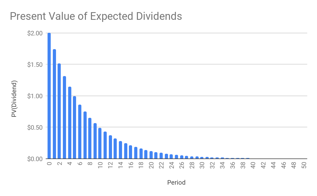
Clearly the further we go in time, the less of an impact a dividend paid at that time will have on the present value of holding the share (and thus the share price). In fact, about 75% of the present value comes from the dividends paid out in the first 10 years, and the next 10 years contributes about another 20%. This means that for a long term investor who plans to hold their share indefinitely, the majority of the value in today’s dollars will be recovered in the next 20 years. The further away the dividend is expected to be paid, the less it is worth today.  

A further assumption of the general dividend model allows us to estimate the share price for a company that we expect will grow. If the growth occurs at a constant rate, then we can apply the Gordon Growth Model (Equation 5). Explicitly we are assuming a constant growth rate and this rate, much like the future dividend values in the other models, is an expectation based on the available information we have on the company. Implicitly we are assuming that expected growth will translate to growth in dividends. Again, looking at the early years of Microsoft, growth in company value does not necessarily result in growing dividend payments.

In general, companies face a tradeoff when it comes to growth. To see this look at the rate of return formula we derived from the Gordon Growth Model (Equation 8). We can see that a company’s share price increases with the expected dividend, [latex]D_1[/latex], and the expected growth rate, [latex]g[/latex].  Therefore, in order to maximise value, a company might wish to increase both [latex]D_1[/latex] and [latex]g[/latex]. However, increasing growth will likely require investment and if the firm spends money on new investments, they have less money available to pay dividends. The firm must find a balance between these two components of the rate of return in order to grow sustainably.

Remember that in the General Dividend Discount model, we make the assumption that the investor plans to hold the share indefinitely.  In other words, the model will take on the form of an infinite sum of dividend payments. We explained that this is a reasonable assumption to apply to the model. Consider an investor planning to sell shares after 5 years, the selling price at year 5 will be the present value of all future dividends beyond year 5. At the same time, the investor would have collected the first 5 years’ dividends. Although the investor will not hold the shares infinitely, the investor will still effectively collect all the future dividends associated with the share. As a result, it is reasonable to assume the infinite sum of dividend payments.

6.6 Summary & Key Formulas

6.6.1 Summary

In this chapter, we focus on share price valuation. Similar to bonds, share price today equals the present value of all future cash flows (dividends) investors will receive. There are two key inputs: the expected dividends and the discount rate. Investors form expectation of future dividends based on current information available. At the same time, the discount rate depends on investors’ assessment of the risk associated with those dividends.

With this basic concept in mind, we introduced the General Dividend Discount Model. We further explored the two special cases of the General Dividend Discount Model. They are the constant dividend model and the constant growth model. As an optional extension, we also discussed how to deal with companies with fluctuations in the growth rate.

For companies that do not pay dividends or have no intention to do so in the near future, we also introduced share valuation using PE ratio. The benchmark PE ratio can be calculated with reference to similar companies or from the historical PE ratios of the company itself. This is particularly useful for young firms such as Microsoft in the 1990s and Tesla today.

6.6.2 Key Formulas