
7 Capital Budgeting Methods
7.1 Introduction
At the end of this chapter, you will be able to:
- explain the importance of capital budgeting decisions
- explain the net present value (NPV) as a capital budgeting method
- calculate the NPV for a project
- explain the payback period as a capital budgeting tool, including its limitations
- calculate the payback period for a project
- explain the internal rate of return (IRR) as a capital budgeting tool
- calculate the IRR for a project using either Excel or a Financial Calculator.
In both your career and your personal life, you are likely to encounter situations where you have to make investment decisions. For example, you may need to decide whether to purchase a property or to keep renting instead. Or, you may decide to become an entrepreneur and need to make decisions on which business opportunities to invest in.
Remember the scenario in which you owned a little coffee-shop? Starting the coffee-shop with your savings was an investment decision, but when running the business and things are going well, you will face more decisions on what to invest in:
- An extra coffee-machine?
- A small baking section?
- A couple of bean bags?
- Another cafe?
Making decisions about what fixed assets to invest in is what we call capital budgeting.
Whether it is a personal or a business investment decision, you would have to conduct some sort of analysis to find out whether it is worthwhile to undertake the investment. Logically, you may say that a financial decision is a good decision if the benefits from the investments exceed the costs incurred. In this chapter, we will discuss capital budgeting tools that can be used to evaluate whether a particular investment adds value to a business or not. That said, the concepts taught here may come in very handy in your own personal investment decisions as well.
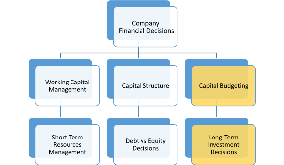
You may remember from Chapter 1 that the three main types of financial decisions a manager has to make are: working capital management decisions, capital structure decisions and capital budgeting decisions (summarised in Figure 7.1).
Working capital management decisions answer questions such as how much short-term resources are needed to keep business running, capital structure decisions deal with questions of how companies raise capital from debt and equity investors, and capital budgeting decisions are related to questions such as which projects or products to invest in to maximise value to shareholders or stakeholders.
This chapter is an introduction to capital budgeting. Capital budgeting is the process of planning and managing company’s long-term investment. Capital budgeting decisions may be driven by several motives.
- One of the motives may be to maintain the current operating capability of the company. Decisions related to this motive include the renewal and replacement of the company’s current production facilities. With this type of investment, companies may operate more efficiently and potentially reduce their costs.
- Another motive for capital budgeting may be to expand the current size of the company. The expansion may include building new production facilities, choosing new projects or introducing new business lines or products. Expansion of the existing business activities may potentially enhance revenues.
- Also, companies may engage in capital budgeting decisions in responding to stakeholders’ demands such as mandatory projects required by government regulations or projects related to corporate social responsibility. While these types of investments may not be related to cost reduction or revenue enhancement, they are still required to keep the business running.
In this chapter, we will focus our discussion on the expansion investments as these are revenue-enhancing, involve more uncertainty and may affect companies more significantly. A similar analysis can be performed for any outlay that provides future benefits to the firm over a period exceeding one year. For some types of decisions, the future benefits may be hard to quantify (such as the goodwill and reputation effects of a principled stand on sustainability), or may be very uncertain or far in the future (such as the benefits derived from reducing the company’s carbon footprint). So, while we will teach you quantitative analysis methods in this chapter, any real-world decision must also consider qualitative and non-quantifiable costs and benefits.
7.1.1 Importance of Capital Budgeting
Capital budgeting decisions are the company’s most fundamental decisions for many reasons:
- Company value - capital budgeting decisions will increase or decrease company value, depending on whether or not the present value of all future cash flows generated from the projects exceed the costs incurred by the project.
- Competition - decisions to take new projects or launch new products/services are necessary for companies to remain competitive. Companies may have little chance of survival without finding new business opportunities and capital budgeting helps to measure the effectiveness of each investment relative to the opportunities available.
- Costs - capital budgeting decisions may involve large cash outlays which are difficult and costly to reverse. Also, given the large amount of resources that might be used in a particular project, accepting one project reduces the company’s opportunity to invest in other projects (opportunity costs).
- Capitalisation - capital budgeting projects often make up the non-current asset portion of the balance sheet. Therefore, these decisions may a have long-term impact on the company.
Concept Check...
7.1.2 Project Classifications
7.1.2.1 Decision Rules
The decision rules we use for capital projects will depend on the relationship of the projects to other investment opportunities the company may have. Project relationships can be classified into the following types:
Independent projects: The decision to accept or reject one project does not directly affect the decision on other projects. This means that if we have enough capital, we could undertake multiple projects as they are independent of each other.
Examples:
- Samsung introducing a new smartphone and the replacement of machinery for a ship building business line. Assuming that Samsung is not capital constrained, accepting the smartphone project will have no effect on the replacement project.
- The establishment of fuel stations and the introduction of online channel for sales (e-commerce) in Walmart. With Walmart’s financing capacity, acceptance of the fuel stations project does not exclude the e-commerce project from consideration.
Mutually exclusive projects: The decision to accept one project prevents the acceptance of other projects. In other words, two or more projects cannot be undertaken at the same time.
Examples:
- Qantas’ decision of purchasing aircraft from either Airbus or Boeing for its longest range flights. The acceptance of aircraft from Airbus will preclude the acceptance of aircraft from Boeing, or vice versa.
- Sony’s decision to locate its largest LCD TV factory either in Europe or in Asia. Once Sony has selected Europe as the factory location, the other possible location is ruled out.
Contingent projects: The decision to accept/reject one project is dependent on the decision to accept or reject one or more other projects. Contingent projects are usually projects that support the success of other projects or become a prerequisite of other projects. Contingent projects may be combined and analysed as a single project.
Examples:
- BHP Billiton also builds facilities such as roads and houses when the company starts its new mining project in a remote area. The project for building the facilities will be accepted only if BHP decides to do the mining project in the area.
- Microsoft’s decision to invest in a data centre was contingent upon the decision of starting its cloud computing business. Investment in data centre is one of the prerequisites for Microsoft’s cloud computing project.
Check Your Understanding...
Match the projects to the project types independent, mutually exclusive and contingent:
Financial managers use project evaluating tools to decide on which project(s) to undertake. These tools include the Net Present Value (NPV), Payback Period, Internal Rate of Return (IRR), Profitability Index and Average Accounting Return (AAR). This chapter will discuss the three most common tools employed by financial managers: NPV, Payback Period, and IRR.
7.2 Net Present Value (NPV)
As stated previously, project evaluation requires cost-benefit analysis. Costs usually occur at the start, when we invest. Benefits from undertaking a project occur after the initial investment has been made. Remember that in finance, cash flows are key, so we measure the project’s future net cash flows (usually estimated to be positive) generated by the project and compare it to the cash outflows from the initial cost (outlay).
NPV compares the future net cash flows and the initial cost by taking into account the time value of money. If, for one reason or another, we do not have to generate a return on our investment, we could just add up the benefits (cash inflows) from a project and deduct the initial cost. However, there is cost associated with using capital. Investors require a return on their investment and even the company has an opportunity cost of investing (and earning a return) elsewhere if it does not need external financing. To account for the time value of money, the net present value evaluates the difference between the present value of the project’s future net cash flows and its current cost (outlay), to understand if the future benefits outweigh the initial costs.
NPV = PV(Future Net Cash Flows) - Initial Cost
NPV = - Initial Cost + PV(Future Net Cash Flows)
When the present value of the future net cash flows generated from the project is greater than the project’s initial cost, then the NPV will be positive. Positive NPV projects generate more than the required return on capital and will thus increase the value of the company and therefore, should be accepted. The present value of future cash flows is computed by discounting the future cash flows at the opportunity cost of capital. This means that if NPV is zero, then the project earns exactly the return that investors (providers of capital) require to take on the risk of the project.
On the other hand, if the present value of the project’s future cash flows are less than the initial cost, then the project will have a negative NPV. Negative NPV projects have a return lower than the investor’s requirement and should be rejected as they decrease the value of the company and consequently, reduce shareholders’ wealth.
NPV Decision Criteria:
NPV > 0 → Accept Project
NPV < 0 → Reject Project
Remember how we computed the value of shares in Chapter 6? The value of a company is measured as present value of future cash flows at an opportunity cost that reflects the risk of those cash flows. Therefore if NPV is positive, the company is earning more than the required return on the project, increasing the present value of the company's future cash flows and increasing the value of the company and its shares.
NPV is considered the best project evaluation tool as it considers the time value of money and is a direct measure of how much the company’s value will increase or decrease by undertaking a particular project.
Note that the NPV decision rule is solely based on the value creation for shareholders. In reality you may consider the value to other stakeholders as well when making a final decision on whether or not to undertake a project.
Concept Check...
7.3 Calculating NPV for a Project
NPV is determined using the discounted cash flow method in which the project’s future net cash flows (cash inflows - cash outflows) are discounted to year 0 and the initial project cost is subtracted from the computed present value of future net cash flows.
[latex]NPV=-CF_{0}+\sum_{n=1}^{N} \frac{CF_{n}}{(1+r)^{n}}[/latex]
7.3.1 NPV Components
In calculating NPV, we need to estimate the initial cost of the projects, the timing and the amount of future cash flows as well as the cost of capital of the project as the discount rate.
- Initial costs - a project’s initial costs are usually incurred in year 0 (upfront) and therefore, the cash outflows are already at present value. For projects with initial costs extend beyond year 0, costs should all be discounted to year 0.
- Future net cash flows - the future net cash flows include cash inflows from revenue generated from the project minus related expenses. In some projects such as replacement projects, the future net cash flows may be cost reductions resulting from the project.
- Discount rate - the discount rate reflects the opportunity cost of the project. That is, the minimum required rate of return of the project given the risk and duration of the project. When a project is relatively risky, the company may require a higher discount rate.
Example
Samsung example
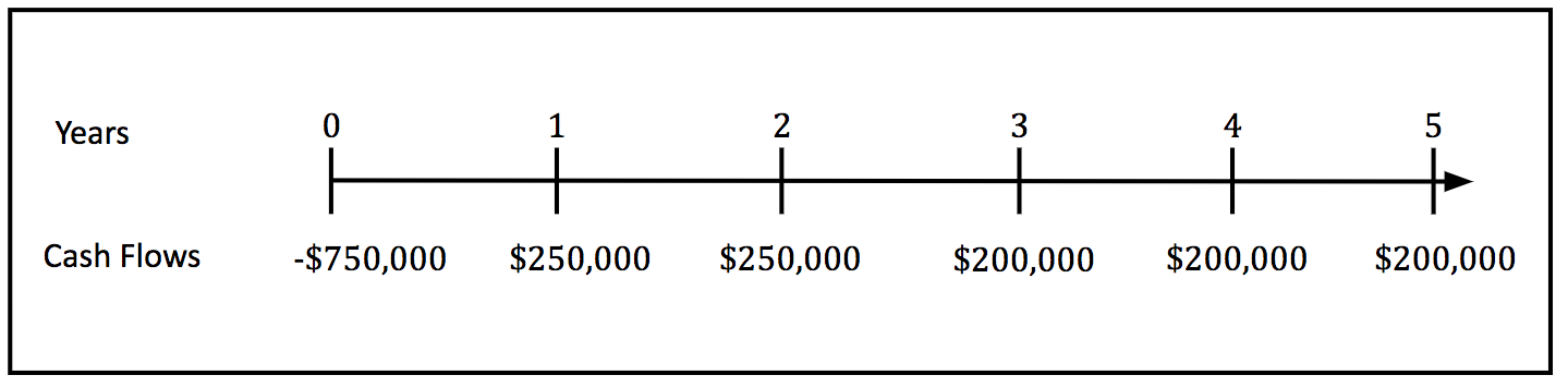
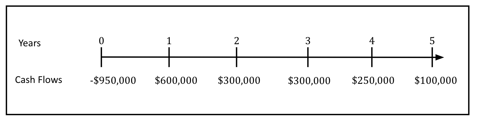
Samsung is considering the launch of 2 different smartphones: smartphone A and smartphone B. Smartphone A will require an initial outlay of $750,000 and is expected to generate after-tax cash flows of $250,000/year for the first 2 years and $200,000 in each of year 3, year 4 and year 5. On the other hand, smartphone B will require an initial outlay of $950,000 and the expected after-tax cash flows generated from smartphone B are $600,000 in year 1, $300,000 in each of year 2 and year 3, $250,000 in year 4 and $100,000 in year 5. Samsung faces an opportunity cost of capital of 10%. If smartphone A and smartphone B are independent projects, should Samsung proceed with any of them? If both projects are mutually exclusive, which project should Samsung choose? (hint: use NPV as the decision criteria).
Solution
Smartphone A
Solving capital budgeting questions can be made much easier by drawing the project’s timeline. The timeline for smartphone A cash flows over its expected life is the following:
Since this question uses the NPV as the decision criteria, we will use the following formula:
[latex]N P V=-C F_{0}+\sum_{n=1}^{N} \frac{C F_{n}}{(1+r)^{n}}[/latex]
The present value of future cash flows is determined by discounting the expected after-tax cash flows from year 1 until year 5. The cost of capital (10%) is used as the discount rate when determining the present value of future cash flows since it is the opportunity cost that reflects the risk of those cash flows. In other words, the project needs to generate at least a 10% return to be a worthwhile undertaking.
Further, the initial cost of the project ($750,000) is deducted from the present value of future after-tax cash flows to get the NPV of the project.
[latex]NPV=-\$ 750,000+\frac{250,000}{(1+0.1)^{1}}+\frac{250,000}{(1+0.1)^{2}}+\frac{200,000}{(1+0.1)^{3}}+\frac{200,000}{(1+0.1)^{4}}+\frac{200,000}{(1+0.1)^{5}}[/latex]
[latex]=-\$ 750,000+\$ 227,272.73+\$ 206,611.57+\$ 150,262.96+\$ 136,602.69+\$ 124,184.26[/latex]
[latex]=-\$ 750,000+\$ 844,934.21[/latex]
[latex]=\$ 94,934.21[/latex]
As the present value of future cash flows ($844,934.21) exceeds the initial cost ($750,000), the project has a positive NPV ($94,934.21). This means this project provides a higher return than what is required (>10%) and the value of the firm increases by $94,934.21 if the project is undertaken.
Smartphone B
Smartphone B project’s timeline is the following:
Using the same step as discussed in smartphone A project, the NPV of smartphone B project is as follows:
[latex]N P V=-C F_{0}+\sum_{n=1}^{N} \frac{C F_{n}}{(1+r)^{n}}[/latex]
[latex]NPV=-950,000+\frac{600,000}{(1+0.1)^{1}}+\frac{300,000}{(1+0.1)^{2}}+\frac{300,000}{(1+0.1)^{3}}+\frac{250,000}{(1+0.1)^{4}}+\frac{100,000}{(1+0.1)^{5}}[/latex]
[latex]=-\$ 950,000+\$ 545,454+\$ 247,933.88+\$ 225,394+\$ 170,733.36+\$ 62,092.13[/latex]
[latex]=-\$ 950,000+\$ 1,251,62.35[/latex]
[latex]=\$ 301,628.35[/latex]
Smartphone B also generates positive NPV ($301,628.35) since the present value of the future cash flows of the project ($1,251,628.35) is greater than its initial outlay of $950,000.
If projects smartphone A and smartphone B cash flows are not related (independent), then Samsung should proceed with both projects as both NPVs are positive. This is because when projects are independent, the company can run the projects at the same time (assuming no capital constraint). So as long as the NPVs of the projects are positive, then undertaking the projects is expected to increase the company’s value.
However, if both projects are mutually exclusive (Samsung can choose either smartphone A or smartphone B due to insufficient demand for both), then Samsung should choose smartphone B as it provides greater NPV ($301,628.35) than smartphone A ($94,934.21). By choosing smartphone B, Samsung will increase the value of the firm more than choosing smartphone A.
Video: Samsung 7.3 (YouTube, 4m35s)
Summary
A firm can measure how much value a project adds to a company’s value by estimating the net present value (NPV) of a project. Net present value refers to the difference between the present value of the project’s future net cash flows and its initial cost (outlay). The project generates a positive NPV if the sum of discounted future cash flows exceeds the initial cost and vice versa. The discount rate is the cost of capital that takes into account the risk of the future cash flows that are expected from an investment. Selecting positive NPV projects also means that the company is earning more than the required return on the project.
7.3.2 Worked Example
Zenzo Inc is considering two energy storage systems for their solar panels. Projects are mutually exclusive. Projected cost and energy savings are displayed below:
|
Year |
Flow System |
Turbo System |
|---|---|---|
|
0 |
-$2,450,250 |
-$1,766,475 |
|
1 |
$810,150 |
$656,253 |
|
2 |
$718,742 |
$501,368 |
|
3 |
$687,543 |
$423,036 |
|
4 |
$554,358 |
$394,358 |
|
5 |
$935,521 |
$604,375 |
The company uses 13.56% to discount such project cash flows. The video below demonstrates computation of NPV and the application of the NPV decision rule.
Video: Worked example (YouTube, 7m34s) (Zenzo Inc part 1)
Video: Worked Example 7.3 in Excel (YouTube, 3m58s) (Zenco Inc Part 2)
Download the Excel template (xlsx, 72KB)
Concept check
You are a financial consultant for Equinox and have been asked for some advice. Equinox Ltd is planning to use marketing services from a digital marketing company. The contract with the digital marketing company requires Equinox to pay an upfront cost of $450,000. Equinox expects that this new marketing strategy will result in additional cash flows of $150 250, $250 650, and $175 000 over the next 3 years.
What is the NPV if the discount rate is 12%?
What if the discount rate is 16%?
Explain how the choice of discount rate influences the NPV and the capital budgeting decision.
7.4 Payback Period - What does it Measure?
How many years does it take to recover my initial investment?
This is what the payback period measures: it is the number of years required for a project to recover its initial cost through future net cash flows. This figure may be useful to understand about your project, but sometimes management selects (sometimes arbitrary) cut-off times, e.g. three years. In that case, all projects that recover their initial cost within the three-year period are accepted while all those that require longer than three years to recover their initial cost are rejected.
Payback period is relatively simple and easy to understand once the cash flows have been estimated. In addition, it is favourable for small businesses as the payback period tends to select projects that generate cash flow more quickly. The small businesses may have fewer resources and need the cash back on their investment to use for other purposes. Another advantage of payback period is that it increases the certainty of the cash flows. This is because the method generally favours projects with a shorter payback period. The longer it takes for the project to recover its initial investment, the greater the uncertainty or risk of the project not providing enough benefits.
Despite its positive features, the payback period has some disadvantages.
- First, it ignores the time value of money, i.e. it treats cash flows equally even though they occur at different points in time. Unlike the NPV that discounts future net cash flows, the payback period simply calculates the sum of the future net cash flows (violating the rule learned in the Time Value of Money module that cash flows can only be compared at the same point in time).
- Second, the cut-off point (eg. three years) is arbitrarily set by the management. Hence, the cut-off point for the decision rule will be highly influenced by judgement rather than an objective basis.
- Third, it ignores cash flows after the cut-off date. This limitation is especially relevant when the payback period is used to compare two projects or more. Payback period tends to choose project with faster initial cost recovery, regardless of the project’s cash flows after the cut-off date compared to other projects.
- Fourth, as payback period favours projects that generate cash inflows sooner than later, it may reject long-term projects such as research and development projects.
Payback Period Decision Criteria:
Payback period < cut-off year → Accept Project
Payback period > cut-off year → Reject Project
Exercises
7.5 Calculating the Payback Period for a Project
Similar to the NPV, payback period calculation requires initial cost and future net cash flow estimates. The payback period can be calculated using the following formula:
[latex]\text{Payback Period}=\text{Years before cost recovery}+\frac{\text {Remaining cost to recover}}{\text {Cash flow during the year}}[/latex]
How this formula works may be best explained with a simple example. Suppose a company proposed a project that requires an initial cost of $50,000. The project is expected to generate cash flows of $15 000, $20 000, $30 000 and $45 000 in the next four years. In this case, the cumulative cash flow after 2 years is $35,000 ($15,000 + $ 20,000) while the cumulative cash flows after 3 years is $65,000 ($15,000+$20,000+$30,000). Hence, the project pays back the initial cost of $50,000 sometime in the third year and the number of years before cost recovery is 2 years.
After 2 years, the project has paid back $35,000, leaving $15,000 to be recovered ($50,000-$35,000), which we call the remaining cost to recover. Further, we need to determine the fractional year when the initial cost is fully recovered by dividing the amount to be recovered ($15,000) with the cash flow in year 3 ($30,000), which is referred to as the cash flows during the year in the formula above. This $15,000 is $15,000/30,000= ½ of the third year cash flow. Assuming that the $30,000 cash flow is paid uniformly throughout the year, the project’s payback period will be 2.5 years.
[latex]\begin{aligned} \text {Payback Period} &=2+\frac{50,000-35,000}{30,000} \\ &=2.5 \text { years } \end{aligned}[/latex]
Whenever a project is estimated to have equal future cash flows each year, let’s say $15,000 for the next four years, then the formula can be simplified into:
[latex]\text{Payback Period}=\frac{\text { Project Cost }}{\text { Yearly Cashflows }}[/latex]
If the project above was expected to generate cash flows of $15,000 for 4 years with an initial cost of $50,000, then the payback period would be:
[latex]\text{Payback Period}=\frac{50,000}{15,000}=3\frac{1}{3}\text{ years}[/latex].
7.5.1 Worked Example
Let’s analyse the Samsung case again. What is the payback period for smartphone A and smartphone B. Which project should Samsung choose if it sets the 3 years as the cut-off year?
|
Year |
Smartphone A Cash Flows |
Cumulative Future Net Cash Flows |
Smartphone B Cash Flows |
Cumulative Future Net Cash Flows |
|---|---|---|---|---|
|
0 |
-750,000 |
-750,000 |
-950,000 |
-950,000 |
|
1 |
250,000 |
-500,0001 |
600,000 |
-350,000 |
|
2 |
250,000 |
-250,0002 |
300,000 |
-50,000 |
|
3 |
200,000 |
-50,000 |
300,000 |
250,000 |
|
4 |
200,000 |
150,000 |
250,000 |
500,000 |
|
5 |
200,000 |
350,000 |
100,000 |
600,000 |
1 -750,000 + 250,000
2 -500,000 + 250,000
Video: Samsung 7.4 example (YouTube, 3m36s)
7.5.1.1 Solution to Worked Example
Smartphone A Payback Period
[latex]\text{Payback Period}=\text{Years before cost recovery}+\frac{\text { Remaining cost to recover }}{\text { Cash flow during the year }}[/latex]
We can find out the number of years before the initial cost is recovered by identifying the year after which the cumulative cash flows turn positive. For Smartphone A, this is year 3. In year 3, only $50 000 is left to recover the initial cost and in the fourth year, a cash flow of $200 000 is expected. Thus the expected payback period is:
[latex]\text{Payback Period}=3+\frac{50,000}{200,000}=3.25 \text {years}[/latex]
Smartphone B Payback Period:
With the same logic, the payback period for smartphone B will be between 2 and 3 years. The exact payback period is:
[latex]\text{Payback Period}=2+\frac{50,000}{300,000}=2.17\text {years}[/latex]
Smartphone B payback period (2.17 years) is shorter than the cut-off year (3 years). So smartphone B should be accepted. On the other hand, smartphone A should be rejected as the payback period (3.25 years) exceeds the cut-off year. Therefore, based on the payback period criteria, Samsung should only proceed with project B. In this case, the decision is the same regardless of whether the projects are independent or mutually exclusive.
Previously we calculated the NPV for two energy saving projects Zenzo Inc is considering:
|
Year |
Flow System |
Turbo System |
|---|---|---|
|
0 |
-2,450,250 |
-1,766,475 |
|
1 |
810,150 |
656,253 |
|
2 |
718,742 |
501,368 |
|
3 |
687,543 |
423,036 |
|
4 |
554,358 |
394,358 |
|
5 |
935,521 |
604,375 |
The following video shows how to calculate the payback period for the Flow System.
Video: Zenzo Inc example 7.4 - Payback of the flow system (YouTube, 5m53s)
7.5.1.2 Worked example PDF
Please download the Zenzo Inc Payback Period for the Flow System (PDF, 718KB) worked example.
Concept Check
What is the payback period for the Turbo System?
Which system should Zenzo choose based on the payback period, if the cut-off is 3.5 years? (remember the projects are mutually exclusive!)
Exercise
Should Melrose Ltd purchase new machinery?
Melrose Ltd is considering to purchase new machinery to increase its production capacity. The cost of the new machinery is $7,270 and the additional cash flows generated from adding the production capacity over the four years are projected to be $2,600, $3,350, $2,850 and $1,150. The company imposes a payback cut-off of 3 years for this project.
If Melrose Ltd uses the payback period as their decision criteria, should it accept this project?
Solution:
The payback period of this project is calculated as follows:
| Year | Smartphone A Cash Flows | Cumulative Future Net Cash Flows |
|---|---|---|
| Year 0 | -7,270 | -7,270 |
| Year 1 | 2,600 | -4,670 |
| Year 2 | 3,350 | -1,320 |
| Year 3 | 2,850 | 1,530 |
| Year 4 | 1,150 | 2,680 |
The cash flows are going to be recovered somewhere between year 2 and year 3, given that there is $1,320 left to recover in year 2, and the cash flows in year 3 are larger than what is needed to recover the investment in full. The exact payback period is calculated as follows:
[latex]\text{Payback Period }=2+\frac{1320}{2850}=2.46\text{ years}[/latex]
Since the payback period of the project (2.46 years) is less than the cut-off year (3 years), the company should proceed with the project.
7.6 Internal Rate of Return (IRR)
7.6.1 What is the Internal Rate of Return (IRR) and What does it Measure?
The internal rate of return (IRR) is a commonly used capital budgeting method, and is the discount rate when NPV = 0. The IRR tells us what return the project is expected to generate. The IRR is intuitively very easy to understand, and we will learn in this chapter how and when we can use it to make capital budgeting decisions.
To solve for IRR, we can use the NPV formula discussed previously and set NPV to zero:
[latex]\begin{aligned} N P V &=-C F_{0}+\sum_{n=1}^{N} \frac{C F_{n}}{(1+r)^{n}} \\ 0 &=-C F_{0}+\sum_{n=1}^{N} \frac{C F_{n}}{(1+I R R)^{n}} \end{aligned}[/latex]
(Remember, [latex]N[/latex] is the life of the project and [latex]n[/latex] refers to each year in turn)
Similar to the yield to maturity in bond valuation, IRR cannot be solved directly. We can use the trial and error approach or spreadsheet function to determine IRR.
The example below illustrates an example of estimating the IRR using trial and error. Suppose a company has a three-year project with an initial cash outlay of $500,000. The company projects future cash inflows to be $100 000, $200 000, and $300 000 for year 1, year 2 and year 3, respectively. The IRR of the project can be estimated using trial and error. With this method we estimate the IRR by trying a discount rate, and then adjust it, until NPV = 0.
Let’s try a discount rates of 7%:
[latex]\begin{aligned}r=7 \%, NPV &=-500,000+\frac{100,000}{(1+0.07)^{1}}+\frac{200,000}{(1+0.07)^{2}}+\frac{300,000}{(1+0.07)^{3}} \\ &=\$ 13,035.05 \end{aligned}[/latex]
A discount rate of 7% results in a positive NPV. We are trying to find out at which discount rate NPV is zero, therefore we have to increase our discount rate (this will decrease NPV). So let’s try a discount rate of 9%.
[latex]\begin{aligned}r=9 \%, NPV &=-500,000+\frac{100,000}{(1+0.09)^{1}}+\frac{200,000}{(1+0.09)^{2}}+\frac{300,000}{(1+0.09)^{3}} \\ &=-\$ 8,265.84 \end{aligned}[/latex]
Now the NPV is negative, this means our estimated discount rate is too high. Now, if we adjust it to 8% and keep making adjustments, we will find that 8.21% is the rate that makes NPV equal to 0.
[latex]\begin{aligned} r=8.21 \%, NPV &=-500,000+\frac{100,000}{(1+0.0821)^{1}}+\frac{200,000}{(1+0.0821)^{2}}+\frac{300,000}{(1+0.0821)^{3}} \\ &=-\$ 18.36 \approx 0 \text { (the discount rate rounded from } 8.2082635 \%) \end{aligned}[/latex]
We can also find the IRR (more easily!) by using a spreadsheet.
VIDEO: Calculating IRR using Excel (YouTube, 58s)
7.6.2 IRR Decisions
IRR calculates the rate of return earned by a particular project. It computes the compound annual rate of return generated by an investment. A project with an IRR that exceeds its required rate of return should be accepted as this implies a positive NPV.
Decisions made using IRR are generally consistent with the decisions based on NPV, but only if we are evaluating independent projects and those projects have conventional cash flows. IRR should not be used in the following cases:
- Non-conventional cash flows
- Ranking mutually exclusive projects
7.6.2.1 Non-Conventional Cash Flows
Non-Conventional Cash Flows are cash flows that have more than one sign change. Thus far, we have had a cash outflow at the start (minus sign) and only cash inflows after (plus sign), which is what we call conventional cash flows. To illustrate non-conventional cash flows, let’s analyse a mining project with the following cash flows. Unlike a project with conventional cash flows that has an initial cash outflow followed by future cash inflows, this project has a cash outflow in year 4 (-$2,250,000). The negative cash flows at the end of the project could be the result of major site restoration.
|
Year |
Cash Flows |
|---|---|
|
0 |
-$1,000,000 |
|
1 |
$800,000 |
|
2 |
$1,000,000 |
|
3 |
$1,350,000 |
|
4 |
-$2,250,000 |
To understand the effect of the cash flows, we will determine NPVs at various discount rates as follows:
|
Discount Rate |
NPV |
|---|---|
|
5% |
-$15,965.57 |
|
15% |
$52,997.95 |
|
20% |
$57,291.67 |
|
30% |
$33,787.33 |
|
40% |
-$12,078.30 |
As shown above, as the discount rate increases from 5% to 15%, NPV changes from negative (-$15,965.57) to positive ($52,997.95). Later, the NPV becomes smaller and turns into negative number again when the discount rate is 40% (-$12,078.30).
The NPV profile below shows that the line crosses the x-axis at two points. In other words, there are two discount rates that make NPV = 0. One at 6.4% and the other at 37.6%. In this situation, there is no correct answer for IRR as we have multiple IRRs.
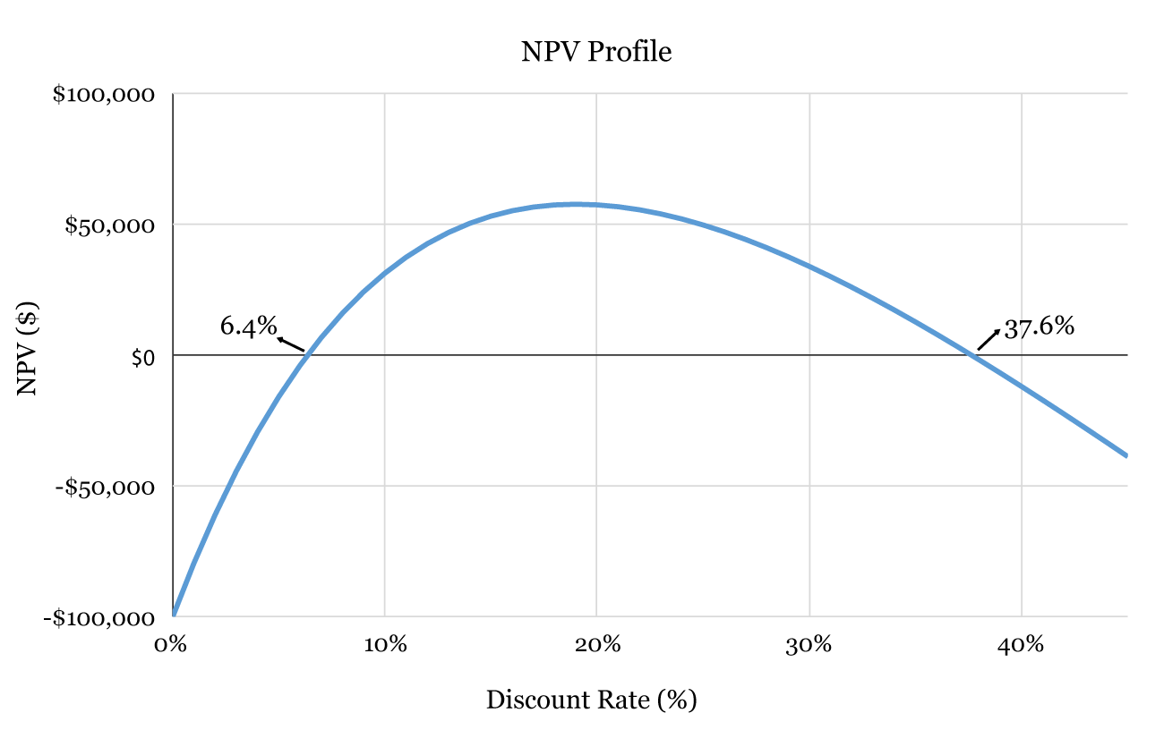
The number of IRRs in a project is equal to the number of cash flows sign changes (positive to negative or vice versa) in the project. In our example, we had two IRRs as we have two sign reversal in the cash flow streams (from -$15,965.57 to $52,997.97 and from $33,787.33 to -$12,078.30).
Ranking Mutually-Exclusive Projects
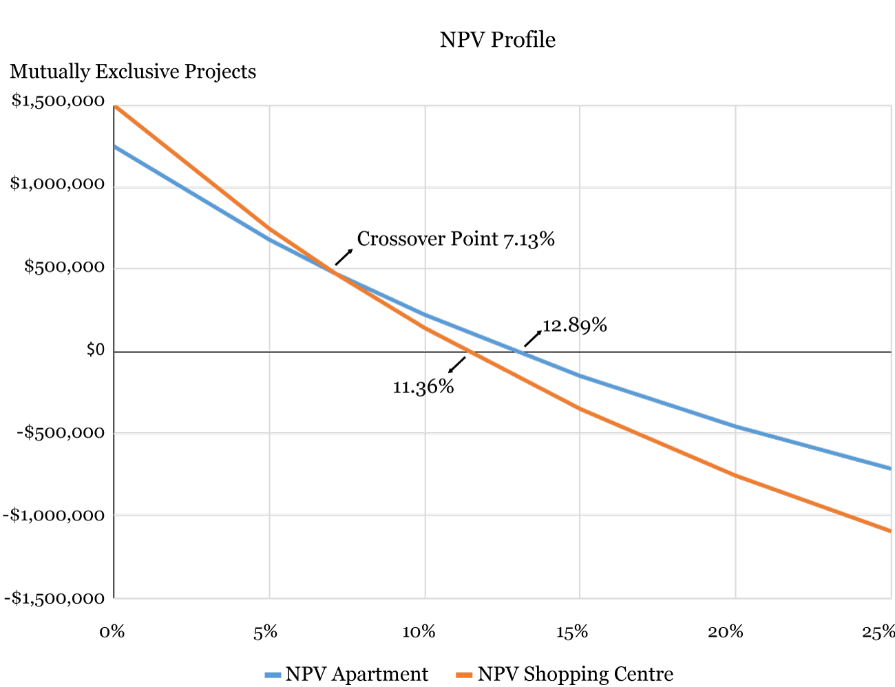
Another problem with IRR is related to mutually exclusive investment decisions. In this case, IRR and NPV may result in a different decision. This is due to the fact that projects are likely to have different scales. Suppose a company is considering whether to utilise its land by either building an apartment or building a shopping centre. The expected cash flows from this mutually exclusive projects are the following:
|
Year |
Apartment |
Shopping Centre |
|---|---|---|
|
0 |
-$3,000,000 |
-$4,000,000 |
|
1 |
$800,000 |
$900,000 |
|
2 |
$900,000 |
$1,000,000 |
|
3 |
$900,000 |
$1,500,000 |
|
4 |
$850,000 |
$1,100,000 |
|
5 |
$800,000 |
$1,000,000 |
The IRRs of the projects are the following:
- [latex]IRR_\text {Apartment} : 12.89%[/latex]
- [latex]IRR_\text {Shopping Centre}: 11.36%[/latex]
If we use IRR as the decision criteria, then we will choose the apartment project because it has a greater IRR (12.89%) compared to the shopping centre project (11.36%). However, if we use NPV, then we may choose the shopping centre project for some discount rates as it has a greater NPV.
Again, to understand the effect of the cash flows from these projects, we will determine NPVs at various discount rates as follows:
|
Discount Rate |
\[NPV_\text{Apartment}\] |
\[NPV_\text{Shopping Centre}\] |
|---|---|---|
|
0% |
$1,250,000.00 |
$1,500,000.00 |
|
5% |
$681,803.17 |
$748,427.62 |
|
7.13% |
$475,171.16 |
$475,171.16 |
|
10% |
$224,556.20 |
$143,836.42 |
|
15% |
-$148,322.27 |
-$348,867.98 |
|
20% |
-$456,082.82 |
-$755,144.05 |
As shown above, the NPVs for the shopping centre are greater than the NPVs for the apartment project when the discount rates are below 7.13% (the crossover point). Therefore, when the discount rate is below the crossover point, the project’s ranking based on IRR and NPV are in conflict.
Generally, the IRR Decision rule is as follows:
IRR Decision Rule:
IRR > Required rate of return → Accept Project
IRR < Required rate of return → Reject Project
But remember that the IRR cannot be used to rank mutually exclusive projects or when cash flows are non-conventional.
Video: IRR 7.6.2 (YouTube, 8m13s)
Exercises
Concept check
Kathmandu Ltd has the following three independent projects. The company’s required rate of return for the projects is 15%. Determine the IRR for each project based on the cash flows listed below and decide which project(s) should be accepted.
|
Year |
Project A |
Project B |
Project C |
|---|---|---|---|
|
0 |
-$35,000 |
-$50,000 |
-$60,000 |
|
1 |
0 |
$15,000 |
$20,000 |
|
2 |
$15,000 |
$15,000 |
$20,000 |
|
3 |
$20,000 |
$20,000 |
$25,000 |
|
4 |
$20,000 |
$20,000 |
$20,000 |
|
5 |
$10,000 |
0 |
$10,000 |
What is the IRR for Project A based on the cash flows listed above?
What is the IRR for Project B based on the cash flows listed above?
What is the IRR for Project C based on the cash flows listed above?
Which projects should be accepted based on the companies required return rate of 15%?
7.7 Summary and Conclusion
7.7.1 Summary
Capital budgeting is one of the most fundamental decisions for modern corporations. Deciding on the right projects to invest in can have profound impact on the company performance, given the capital investment typically involves large amount of resources and not reversible once the investment is made. There are three different types of projects, namely, independent projects, mutually exclusive projects and contingent projects.
In this chapter, we have learnt three common methods in evaluating capital investment projects. The first method is NPV, which compares the future net cash flows and the initial cost by taking into account the time value of money. The decision rule is to accept projects with positive NPVs if they are independent. When projects are mutually exclusive, then the project with highest NPV should be accepted.
The second method we have learnt is payback period, which measures the number of years required for a project to recover its initial cost through future cash flows. The decision rule is to accept projects with payback periods less than the cut-off times set by the management. For mutually exclusive projects, the project with shortest payback period should be accepted. The drawbacks of payback period includes the omission of time value of money, the arbitrary cut-off point, the omission of cash flows after the cut-off date, and the rejection of long-term projects such as research and development projects.
The third method is the IRR, which calculates the discount rate that makes the NPV equal to 0. The IRR tells us what return the project is expected to generate, and we should projects with IRRs higher than the hurdle rates set by the management. For mutually exclusive projects, the project with the highest IRR should be accepted. However, IRR should not be used when there is non-conventional cash flows or when ranking mutually exclusive projects with different scales.
7.7.2 Key Formulas
NPV Formula:
[latex]N P V=-C F_{0}+\sum_{n=1}^{N} \frac{C F_{n}}{(1+r)^{n}}[/latex]
[latex]C F_{0}=\text {initial cost (including discounted project costs after year 0)}[/latex]
[latex]C F_{n}=\text {net cash flow in period $n$, where n} =1,2,3, \ldots \text {N}[/latex]
[latex]\text {r= the discount rate (cost of capital)}[/latex]
[latex]\text {$n=$ the project's estimated life}[/latex]
Payback period formula:
[latex]\text { Payback Period = Years before cost recovery }+\frac{\text { Remaining cost to recover }}{\text { Cash flow during the year }}[/latex]
IRR Formula:
[latex]0=-C F_{0}+\sum_{n=1}^{N} \frac{C F_{n}}{(1+I R R)^{n}}[/latex]
