
9 NPV – Modelling and Analysis
9.1 Introduction
At the end of this chapter, you will be able to:
- estimate the sensitivity of an output to a change in an input
- estimate the NPV break-even point for a project
- explain sensitivity analysis, scenario analysis, and simulation analysis and describe how they are used to evaluate the risks associated with a project
- construct a capital budgeting analysis in Excel
- evaluate a proposed capital budgeting project.
In the previous two chapters we learnt how to identify relevant cash flows to use in project analysis, and how to use capital budgeting tools. When calculating the NPV we relied on (well-informed) estimations of what the cash flows would be if we undertook the project. We were given estimations on how much sales a new project would generate, what the costs would be, what the tax rate would be, and so forth. But how sure are we of these estimations? Is it possible to accurately estimate all variables? Do you think that any project's cash flows are estimated 100% correctly? Probably not. In reality, the estimations are almost certainly going to be different from what actually occurs. So does this mean our analysis is useless? Or is there some way we can account for this uncertainty?
Of course, our analysis so far has not been useless – the estimations we made are based on information available to us at the time, and are our “best guess”. It is a baseline for us to understand the viability of a project.
We are looking at different types of risks, with the aim to understand how the change in an input (i.e. assumption) affects the feasibility of a project. If the change in an input has a great impact on the attractiveness of the project, then more time should be spent investigating the variables' expected outcome.
This chapter will cover three common forms of risk analysis:
- Sensitivity analysis
- Scenario analysis
- Simulation analysis
9.1.1 Practical example - YoGo Technologies
This section revises the computation of NPV in detail. Having completed Chapter 8, you should try to do the NPV analysis yourself, then check against the solution. This is a good test to see if you have understood Chapter 8.
The problem: YoGo Technologies is investigating a potential new product that will generate a net revenue of $20 per unit. The expected sales are 5,000 units per year, for 5 years. Production equipment will cost $200,000 and will be depreciated straight-line over 5 years, to 0. After 5 years the equipment will be sold for $50,000. The company tax rate is 30%, and the required return is 10%. What is the NPV of the project?
Below provides a recap on calculating NPV, if you have been keeping up you probably do not need it. After the text solution, there's a video of the solution as well - jump there if that's how you prefer to learn.
9.1.1.1 RECAP – calculating cash flows
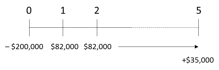
As you may recall, typically the timeline of a project’s cash flows looks like this:
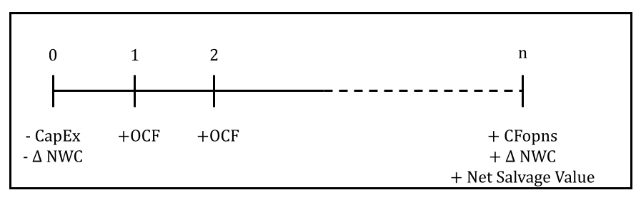
We start with the capital expenditure or initial cost. This is the initial outlay (–CapEx), reflecting that we made an investment into something. Sometimes we also have to invest in additional net working capital (- Δ NWC). Then, if all goes well, we start receiving cash flows from operations (+OCF) for the life of the project. For example, when we start selling products, we will have cash inflows. We continue having these cash flow from operations for the life of the project. At the end of the project, at year ‘n’, we usually recover the investment in net working capital if we made any (+Δ NWC). Sometimes, we are able to sell the equipment at the end, which will also return a cash inflow. In this case, we have to calculate the net cash inflow from this sale, which is indicated as the net salvage value.
Let’s start with the cash flows from operations. As we did in Chapter 8, we use a basic income statement to identify the cash flows.
Step 1: Cash flows from operations
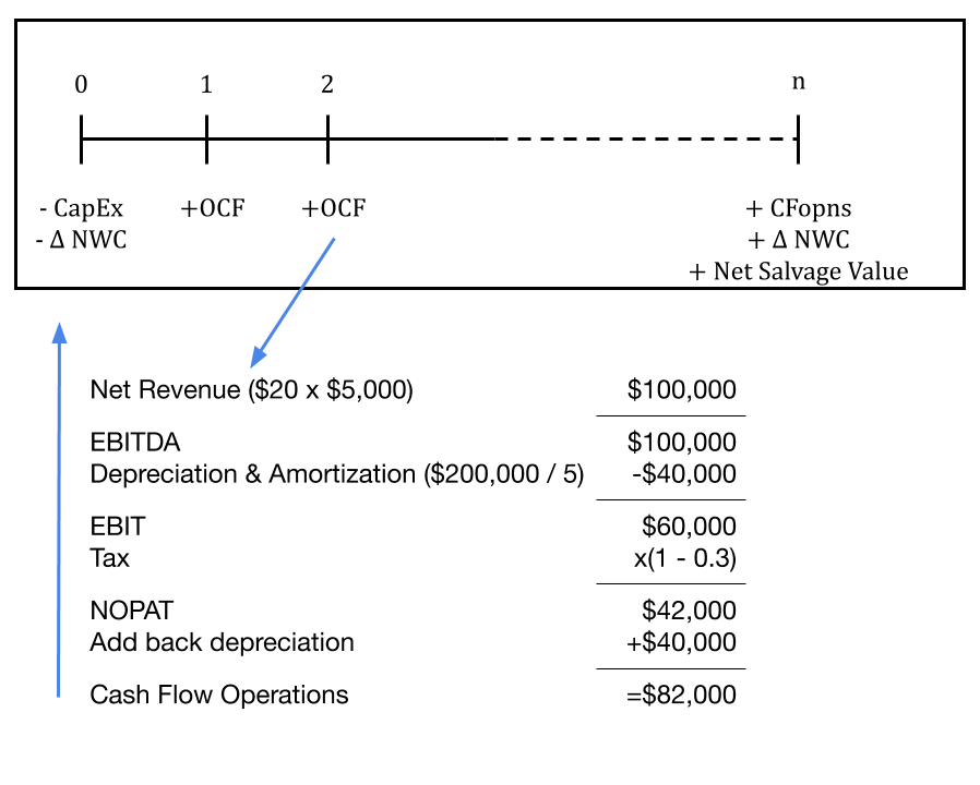
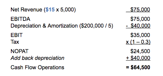
In this exercise, we have the net revenue per unit sold, which is the revenue minus the costs of goods sold, and this gives us the gross profit per unit. To calculate the total net revenue, we multiply the net revenue per unit, which is $20, by the number of units we are selling, which is 5,000 units; $20 x 5,000 = $100,000. Note that here we already counted the costs of goods sold and we do not have any other expenses remaining. In general, we could have some fixed costs to be calculated, which would add up to EBITDA. In this simple example, the $100,000 is the EBITDA. What comes after EBITDA? We have to calculate the depreciation and amortisation. In this example, we only have depreciation, but no amortisation. Depreciation is calculated as the initial cost divided by useful life of the equipment you are investing in. In this case, this is $200,000 divided by 5, which is $40,000. This is our annual depreciation.
Focusing on the annual cash flow, we will calculate the EBIT, which is $100,000 minus the $40,000, so it is $60,000. Next, we have to consider interest and tax. It is important to note that even if we had an interest expense, we would not include it in this statement because it is not an operating cash flow and it does not affect the amount of tax we have to pay. In this example, we do have a tax rate of 30%. We can find the Net Operating Profit After Tax (NOPAT), by multiplying the EBIT amount by ‘1 minus the tax rate’, so (1 – 0.3), giving us $42,000.
Do we have the cash flows from our operations? Not yet! We still need to add back depreciation and amortisation. This is $42,000 plus the depreciation of $40,000, adding up to $82,000, which are the cash flows from operations. This amount is the actual cash we generate each year, where we are undertaking this project. This is step 1.
Now we move on to Step 2.
Step 2: Identifying the cash flows at the start of the project.
There is no investment in net working capital, but we do have an initial capital expenditure that we have to spend to start the project. In this example, it is $200,000.
Step 3: Identifying the cash flows at the end of the project.
In step 3, there is no net working capital recovery as we didn’t invest in any, but we do receive a cash flow from selling our production equipment. To find out exactly how much we calculate the net salvage value;
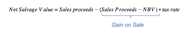
To unpack this equation, let’s start by calculating the net book value (NBV). In this case, this will be 0, because we depreciated it to 0. We then have the proceeds, which is the amount we are receiving from selling the assets. In this example, this will be the re-sale value of $50,000. In other words, this is the cash we are receiving, but we have to make an adjustment for the tax we may have to pay. Combining everything together, we are receiving $50,000 on our book value, which is worth 0, meaning that we are making a gain on sale of $50,000, over which we still have to pay 30% tax. Therefore, we multiply the $50,000 by the tax rate of 30%. Overall, the net cash we are receiving from selling this asset is $35,000.
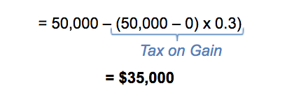
In other words, we receive $50,000, but we have to pay $15,000 worth of tax, which is the tax on gain. What happens if you make a loss on sale? This means you would get tax back. This is because the loss on sale can be used to offset other taxable income, reducing the tax payment. Effectively, we are getting some tax back in addition to our sales proceeds.
Now that we have calculated these values, we can redraw the timeline with specific numbers.
At time 0, we have -$200,000 and we have an expected cash flow of $82,000 for 5 years. In addition to that, at the end, we will also receive the $35,000 from selling the asset.
Combining this together, we will calculate the NPV. We hope you remember what NPV tells us – if the NPV is positive, it means that the project adds value to the firm, so the company increases in value. In other words, the project generates a higher return than the cost of capital we are discounting at. In this example, we are using the discount rate of 10% to calculate the present value. Therefore, if the NPV is positive, it means that the project is generating more than 10% and thus adds value to the firm.
Firstly, remember the formula from Chapter 8?
[latex]N P V=-C F_{0}+\sum_{n=1}^{N} \frac{C F_{n}}{(1+r)^{n}}[/latex]
For the OCF we can use the annuity formula, resulting in:
[latex]\begin{aligned} \mathrm{NPV} &=-\$ 200,000+\$ 82,000 \times\left(\frac{1-\frac{1}{1.10^{5}}}{0.10}\right)+\frac{\$ 35,000}{1.10^{5}} \\ &=-\$ 200,000+\$ 332,576.76 \\ &=\$ 132,576.76 \end{aligned}[/latex]
This can also be done in excel, below the solution is a link for the Excel template and video to solve this way.
By using either the manual calculation or excel, we will get an NPV of $132,576.76. This means that if the company proceeds with the project, it will make more than 10% of what is required and will add $132,576.76 to the value of the business.
The following two videos go through this solution in detail, first using a pen and calculator, and second using a spreadsheet program.
Video: NPV Calculation (YoGo) (YouTube, 13m19s)
Download the Excel template (XLSX, 11.6KB).
Video: NPV Calculation in Excel (YoGo) (YouTube, 10m38s)
Everything so far was covered in Chapter 8, and now we are ready to start conducting a Sensitivity Analysis in the next section.
We are looking to answer: What happens if the net revenue changes? How would that affect the NPV? How much can net revenue change for the project to be still beneficial?
9.2 Sensitivity analysis
Sensitivity analysis is the simplest, most basic form of risk analysis, which shows how sensitive an output variable is to a change in an input variable. With respect to capital budgeting, we are often interested in examining the sensitivity of the output from an analysis, such as the NPV estimate, to changes in the input variables.
[latex]\text{Sensitivity (slope)}=\frac{\Delta NPV}{\Delta Input}[/latex]
Where “input” can be any variable or assumption that has an impact on NPV, such as sales volume, interest rates, or production costs.
An analyst might look at how a project’s NPV changes if there is a decrease in the value of individual cash inflow assumptions or an increase in the value of individual cash outflow assumptions. For example:
- What happens if the sales of a company decrease?
- How will it affect the NPV?
- Or what happens if the costs increase?
- How much can the costs increase before it becomes unattractive to take on the project?
We can calculate this by looking at how a certain change in a given input will affect NPV. With sensitivity analysis, we’re looking at how a single input variable affects NPV.
9.2.1 Calculating sensitivity
Calculating the sensitivity of NPV from changes in net revenue gives us an exact number of how much NPV changes when net revenue changes by one unit. We can simply re-calculate the new NPV if net revenue goes up by one, or we can pick any new number of net revenue and the sensitivity formula gives us the same result (unless there is a non-linear relationship).
To see how this works, let’s assume the new net revenue is $15 dollars per unit. The new cash flows from operations calculation with this input would look like this resulting in $64,500.
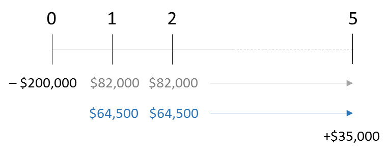
This means that with a net revenue of $15 per unit, we would have an annual cash flow of operations of $64,500. In comparison with the original timeline, the initial capital expenditure and the net salvage value will stay the same, but the cash flow operations each year will need to be updated. Under the new scenario, the timeline will look like this. Overall, the only value that changes is the cash flows from operations.
What is the NPV under this new scenario?
[latex]\mathrm{NPV}=-\$ 200,000+\$ 64,500 \times\left(\frac{1-\frac{1}{1.10^{5}}}{0.10}\right)+\frac{\$ 35,000}{1.10^{5}}[/latex]
By using either the manual calculation or excel, our equation would be: minus (-) $200,000, plus (+) the $266,237.99, which gives us the present value of $66,237.99.
What does this mean for the project? In this new scenario, although we are making less money per unit sold, the NPV is still positive, and it is still worth undertaking this project.
Similarly, we can compute NPV for various changes in assumptions. Here are the results of those computations:
| Variable of Interest | Value | NPV |
|---|---|---|
| Base Case | 132,576.76 | |
| Net Revenue per unit | $15 | 66,237.99 |
| Units sold | 4,000 | 79,505.75 |
| Equipment salvage value | $45,000 | 13,403.54 |
While these numbers are informative, it would be even better to be able to answer the question “How much does a 1 unit change in input change NPV?” This is the purpose of sensitivity analysis. It helps us see which inputs make the greatest difference to the profitability of a project. This next video demonstrates the computation of sensitivity.
[latex]\text{Sensitivity (slope)}=\frac{\Delta NPV}{\Delta Input}[/latex]
In the sensitivity analysis, we calculate the change in NPV per unit change in the inputs. The aim of the sensitivity analysis is to analyse how the NPV changes from the change in net revenue per unit (S1 = Scenario 1 and S2 = Scenario 2).
[latex]\text{Sensitivity}=\frac{NPV_{S 1}-NPV_{S 2}}{NR_{S 1}-NR_{S 2}}[/latex]
The change in net present value is calculated as the old NPV, $132,576.76 minus the new NPV value of $66,237.99, divided by $20 per unit minus $15 per unit. This calculation will give us the result of $13,267.75.
[latex]\text{Sensitivity}=\frac{NPV_{20}-NPV_{15}}{NR_{20}-NR_{15}}=\frac{\$ 132,576.76-\$ 66,237.99}{\$ 20-\$ 15}=\$ 13,267.75[/latex]
What does this number mean? This number shows us that if our net revenue per unit goes up by $1, our NPV will increase by $13,267.75. It is a positive relationship, meaning that if our net revenue per unit increases, the NPV also increases. Similarly, if the net revenue per unit decreases by $1, then the NPV also decreases by $13,267.75. On the contrary, focus on costs would most likely deliver a negative relationship, meaning that a $1 increase in cost would decrease the NPV by a certain percentage.
Following this logic...
What happens if the net revenue per unit (=dollar) decreases by $7?
In this case, the NPV would decrease by 7x the amount of $13,267.75, so by $92,874.28.
We can also use the sensitivity figure to find out by how many dollars our net revenue can change before we “break-even” (NPV = 0), meaning changing it any further would make the project unfeasible.
Our original estimate of a net revenue of $20 resulted in an NPV of $132,576.76. We can divide the NPV by the sensitivity to find net revenue break-even point;
[latex]\begin{aligned}\text{ Breakeven net revenue }&=\text{ net revenue}_{20}-\frac{N P V_{20}}{\text{ Sensitivity }_{ net revenue}}\\&=\$ 20-\frac{$132,576 .76}{$13,267.75}\approx\$ 10.01\end{aligned}[/latex]
This means that at a revenue of $10.01, the project has an NPV of 0 and breaks even. If net revenue is any lower than $10.01, the project will reduce the value of the firm.
Understanding the meaning of the process and the number gives you the ability to interpret how a certain output would change as a result of an input change. Remember that inputs in a project are only estimations and are affected by a number of internal and external factors. It becomes essential to understand how a certain variable change will influence the whole project, as this is an indication of risk. This means that the higher the sensitivity to a certain change in input, the more it is exposed to significant risk from this input changing. So, the higher the sensitivity of NPV to a given input, the more important it will be to estimate that input accurately.
[latex]\text{Sensitivity (slope)}=\frac{\Delta Output}{\Delta Input}[/latex]
The generic formula of sensitivity analysis provides a way to interpret what happens to variable X in the case of a change in variable Y. We used NPV in the previous sensitivity analysis, but we could also be interested in what happens to the Operating cash flows given a certain input change. It is dependent on the context of different scenarios to decide which variable change is best to assess the impact on another important variable. It is common to analyse what happens to the NPV as a result of an input change because, ultimately, this is the method that shows whether a project is worthwhile or not.
In the next video, we will show how to compute the NPV numbers in the table above using Excel. You can use the spreadsheet you created in the previous unit, or you can use this spreadsheet: YoGo-Template - Sensitivity.xlsx. Note: there is a small mistake in the video, it should be; there is a positive relationship between salvage value and NPV (if salvage goes up, NPV goes up)"
Video: Sensitivity analysis (YoGo)
9.3 Scenario Analysis
With sensitivity analysis, we were looking at each input in isolation. However, in the real world, several inputs are subject to change and input are often related to each other. For example, if we raise the price of our new product, this will often result in a decrease in demand for the product.
Analysing price separately from the number of units sold doesn’t really make sense. For scenario analysis, we create various “scenarios”, which are combinations of several inputs or assumptions. We might have a high price scenario that includes higher than expected prices, but lower than expected demand.
The expected or most likely combination of inputs is called the base case scenario. Once we have a base case, we can consider the risk of alternative scenarios. We might define a best-case scenario that includes expected inputs in the event that the economy is booming, or demand for our new product exceeds expectations. And we might define a worst-case scenario with values we would expect if the economy were to fall into recession or if our new product were to be particularly unpopular.
When evaluating the various scenarios, it is important to consider the likelihood of each scenario actually occurring.
The following example provides an overview of an automated vertical food production system, under three different scenarios; strong, expected and weak economic conditions (see table below). It compares the unit sales, unit prices, unit variable costs and NPV in each scenario. For example, you could assume to be selling more at a higher price in strong economic conditions, but also pay higher costs, and vice versa in a weak economy.
|
Economic Conditions |
Unit Sales |
Unit Price |
Unit Variable Costs |
NPV |
|---|---|---|---|---|
|
Strong |
38,500 |
$240 |
$110 |
$272,853 |
|
Expected |
35,000 |
$220 |
$95 |
$153,688 |
|
Weak |
28,000 |
$190 |
$90 |
$(117,523) |
Considering the numbers, with NPV being negative under the worst-case scenario, whether one would undertake this project depends on the person’s risk aversion and the probability for each of the scenarios. It is a matter of question to evaluate how likely it is that the project would deliver the worst-case scenario results. Therefore, utilising the knowledge of this data, the decision becomes dependent on one’s subjective assessment of the probability and risk preference.
9.3.1 Conducting a Scenario Analysis in Excel
Assume that YoGo has identified the following scenarios:
|
Inputs |
Base Case |
Best Case |
Worst Case |
Low Demand |
High Demand |
|---|---|---|---|---|---|
|
Net Revenue |
$20 |
$22 |
$18 |
$19 |
$21 |
|
Sales (units) |
5,000 |
7,500 |
2,500 |
3,500 |
6,500 |
|
Initial Cost |
$200,000 |
$200,000 |
$200,000 |
$200,000 |
$200,000 |
|
Useful Life |
5 |
5 |
5 |
5 |
5 |
|
Salvage |
$50,000 |
$65,000 |
$10,000 |
$50,000 |
$50,000 |
|
Tax rate |
30% |
25% |
35% |
30% |
30% |
|
Discount rate |
10% |
9% |
11% |
10% |
10% |
The first step of conducting a scenario analysis is to calculate the NPV under each scenario. This can be done manually, but is a lot easier in excel. If you want to practice calculating NPV's manually, it would be a useful exercise to calculate the NPV under each scenario and then check with the spreadsheet calculations if you have done it correctly.
The following video will show how to conduct the scenario analysis in excel.
Video: Scenario Analysis in Excel (YouTube, 7m13)
If you have followed the previous videos and have been amending your spreadsheet according to the instructions, you can continue using your spreadsheet. Alternatively, you can use this spreadsheet: YoGo-Template - Scenario (XLSX, 52KB)
9.4 Simulation Analysis
Previously we looked at Scenario and Sensitivity analysis. We have seen that scenario analysis is a more comprehensive analysis than sensitivity analysis because it considers the relationships between the input variables. What it doesn’t explicitly consider is the probability of any given scenario occurring. If we really want to get an idea of the risk of a project, it would be useful to be able to generate a probability distribution for NPV. This is what simulation analysis aims to do. The idea is to look at the probability distributions of the underlying inputs as well as the relationships between those inputs (correlation in statistics). These inputs are fed into a computer to generate a probability distribution for the output, or NPV. The computer uses random number generators to create thousands of equally probable sets of input variables. NPV is computed for each set of inputs to get thousands of equally probable NPVs. The mean (average) and dispersion (standard deviation) of those NPVs gives us an idea of the risk of the project.
9.4.1 Conducting Simulation Analysis in Excel
9.4.1.1 YoGo technologies simulation analysis
The first step in conducting a simulation analysis is simulating what our inputs are likely to be. When simulating the input variables, we usually assume a normal distribution. That is, it is equally likely that a variable is "x" higher or lower than expected. The basic process is to identify the best estimate of your input variable, and then identify the likelihood of your input being different. The best estimate is what we refer to as the mean, and the standard deviation is an estimate of how much we think the variable may be different to our best estimate. This is best illustrated with an example:
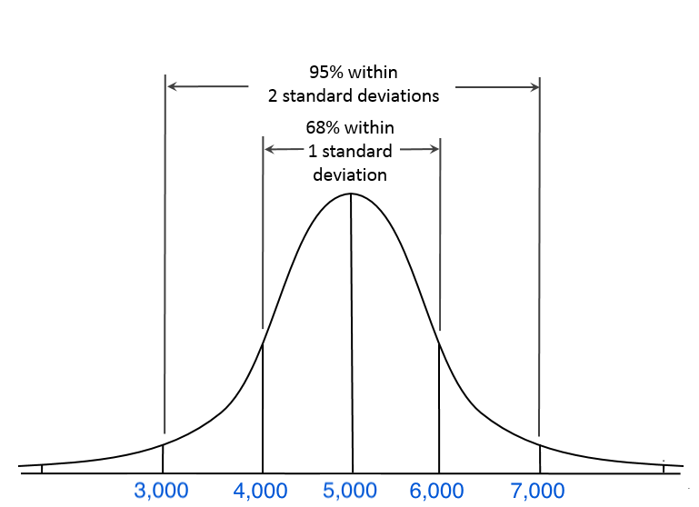
Let's say our best estimate of the units sold is 5,000 (the mean) and we estimate a standard deviation of 1,000 units. This means that we estimate that there is a 68% chance that our sales will be 1,000 units higher or lower than 5,000 and a 95% that it will be two standard deviations away (1,000 x 2= 2000) from the mean. Basically we estimate that the distribution of our unit sales looks like this:
DISTRIBUTION UNIT SALES
We can tell Excel that the distribution looks like this, and then Excel can simulate possible outcomes based on this function.
Second, we can indicate the distribution of another variable of interest, such as net revenue. We can also tell Excel how the variables impact each other by including a correlation variable: there is generally a strong negative relationship between the two variables (if net revenue goes up because of a higher price, sales usually go down). Note that in the next chapter (Chapter 10) we will spend a little bit more time on standard deviations and correlations, for now it is just important to understand intuitively how the simulation analysis works and how it can help making informed decisions.
The following video shows how to conduct a simulation analysis in Excel.
Video – Simulation analysis YoGo.
If you have followed the previous videos and have been amending your spreadsheet according to the instructions, you can continue using your spreadsheet. Alternatively, you can use this spreadsheet: YoGo-Template - Simulation (XLSX, 480KB)
9.5 Summary and Conclusion
9.5.1 Summary: Comparing Risk Analysis Methods
The table below compares all the risk analysis methods.
| ? | Sensitivity Analysis | Scenario Analysis | Simulation Analysis |
|---|---|---|---|
| Input | Change assumption for one variable at a time | Combinations of inputs, where the values are expected to be related (e.g. price and volume) | Random draws from probability distribution of input(s), where inputs may or may not be related |
| Output | Sensitivity output (e.g. NPV or cash flow) to changes in one variable | What IF - how output (e.g. NPV or cash flow) will change IF a given scenario eventuates | Frequency distribution of output (e.g. NPV or cash flow) |
| What Do We learn? | Which forecasts to refine - or which assumptions drive value | If we can choose scenario: which is best. If scenarios are based on external environment: gives us an idea of risk. | Expected value and/or risk (variation) in output (e.g. NPV or cash flow) |
The sensitivity analysis changes the assumption for one variable at a time and it looks at the sensitivity of the output to changes in one variable. It gives a basic understanding of which forecasts to refine or which assumptions drive value. For example, if your NPV is the most exposed to the number of products a company sells, then it becomes a relevant factor to analyse.
In scenario analysis, there is a combination of inputs that change, where the values are often related, for example, the price, the volume and the tax. Essentially, it is a ‘what if’ analysis, referring to certain situations and showing what would happen to the NPV, in the best-case scenario, for example. Sometimes these scenarios are based on economic conditions or other external factors and conditions that are outside of the company’s control. This analysis provides an idea of the risks a project could be exposed to, should the external conditions change.
Lastly, simulation analysis uses a random number from the probability distribution, where inputs may or may not be related and the output delivers a frequency distribution of outputs. This shows how the NPV would change in the thousands of different cases. In other words, we can predict the expected value of the NPV, which would be represented in a sequence of different values.
9.5.2 Key Formulas
Sensitivity analysis:
[latex]\text {Sensitivity (slope)}=\frac{\Delta\ { Output }}{{\Delta\ Input }}[/latex]
