
5 Activity 5 – Standard and Hierarchical Multiple Regression in jamovi
Last reviewed 19 December 2024. Current as at jamovi version 2.6.19.
Overview
In this section we introduce multiple regression analysis procedures. We will conduct these in jamovi. Two kinds of multiple regression are performed, standard and hierarchical. The differences in their output will be highlighted. The aim of this activity is to develop a conceptual understanding of the issues involved in analysing multiple continuous variables, and some of the considerations necessary to interpret the output.
Learning Objectives
- To introduce the jamovi procedures for performing multiple regression analyses
- To highlight the differences between standard (simultaneous) and hierarchical methods in multiple regression analyses
- To gain practice at writing up the results of standard and hierarchical multiple regression analyses
Standard Multiple Regression
In a standard multiple regression, predictors are entered into the model simultaneously, i.e., all together in one “step” or “block”. With a standard multiple regression design, we are able to examine two separate yet related aspects of our data. The first is the overall model. This looks at the total proportion of variance in the criterion that is explained by the model (i.e., all the predictors collectively). For this, we look to the R2 value. The second aspect we can look at is unique predictors. Here we examine the unique proportion of variance explained in the criterion by each individual predictor. This value is given by sr2.
Figure 5.1
Contribution of the Overall Model (R2; Left Panel) and Individual Predictors (sr2; Right Panel) in the Explanation of the Criterion Variance
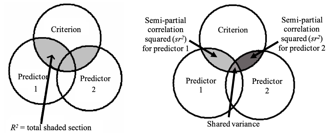
Note. For the right panel, “shared variance” is the variance explained in the criterion shared by both predictors. This is calculated as: Shared variance = R2- sr2predictor1 - sr2predictor2.
Imagine that weight was our criterion in this analysis, and we wanted to predict people's weight based on their height and age. See the Venn diagram below:
Figure 5.2
Venn Diagram of Covariance between Weight, Age and Height
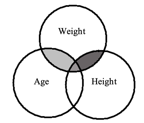
The shaded areas represent the proportion of variance in weight that is shared with variance in height and/ or age (R2) – that is, the extent to which they vary together. This quantity is associated with our correlation coefficient (in this instance the multiple correlation coefficient R). It is our wish to test this quantity for significance in our analysis.
Individual Predictor Statistics
In addition to looking at multiple predictors collectively in a regression analysis, it is sometimes useful to consider the variables individually. This allows us to see how each contributes to the explanation of variance in the criterion. For instance, we might want to know how height and weight are related, independent of how old you are. In order to answer this type of question, we need to look at each variable controlling for the influence of the other predictor variables in the analysis. While there are a number of individual contribution statistics [i.e., b, β, t(df), p, 95% CI, pr2, sr2], only two speak to the unique variance explained by a predictor. These are: partial correlation squared (pr2), and semi-partial correlation squared (sr2). In contrast, b and β indicate the direction of effect (rather than variance).
Partial Correlation Squared (pr2)
To visualise what is meant by partial correlation squared, consider the following Venn diagram. In this, we present the predictor of height, and weight is our criterion.
Figure 5.3
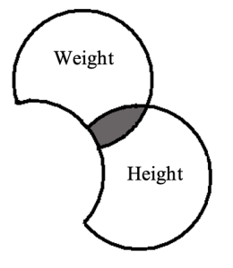
For partial correlation squared (pr2), we remove from each variable (i.e., both the predictor and criterion) the variance (i.e., overlap) which they share with age (second predictor).
The shaded portion, therefore, represents the overlap in variance between height and weight which is not shared with variance in the other predictor variable age. We will look at how this value is calculated later in this booklet. NB: In write-ups the ‘partial’ correlation (i.e., pr) is squared to create the effect size measure and reported as pr2.
Note that the variance for weight (criterion) is no longer represented as a complete circle. This illustrates that partial correlation squared is expressed as the proportion of remaining (i.e., residual) criterion variance that is explained by a predictor (as opposed to its original 100% variance to be potentially explained).
Semi-Partial Correlation Squared (sr2)
To understand what is meant by semi-partial correlation squared, consider another modified Venn diagram.
Figure 5.4
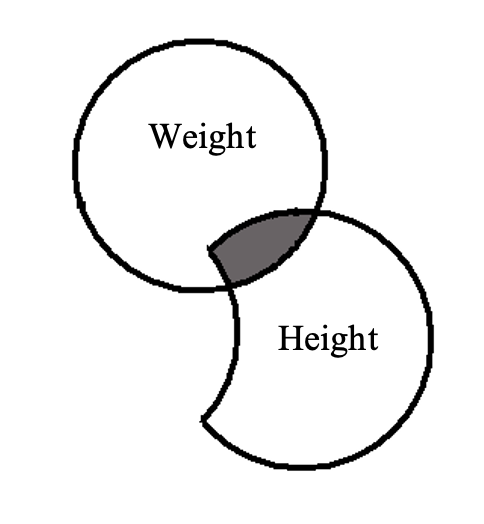
In this instance, the squared correlation is still represented by the shaded area, but the shared variance is expressed as a proportion of the total variance in the criterion variable (weight) that is explained by the predictor (height). Thus, semi-partial correlation squared tells us how much of the total variance in people's weight we can explain on the basis of their height, once the covariance between height and age (i.e., the overlap between just the predictors) has been removed from the equation. NB: in write-ups the semi-partial correlation (sr) is squared to create the effect size measure, and reported as sr2.
Note that in multiple regression, we are still dealing with a model that is created to fit the data. It is like the “line of best fit” in a simple regression, but because we are now dealing with more than one predictor, it gets more complicated. Now it’s like a “plane of best fit” in three-dimensional space. Due to this, the beta (β) weights from the regression equation for each variable are also a measure of the variable’s relative importance. That is, the higher the β value (regardless of direction), the more important that predictor is. Note though, that if you want to compare the strength of two independent predictors, you test for differences in the strength of the contributions of independent predictors using Fisher's z tests of the partial correlations.
Hierarchical Multiple Regression
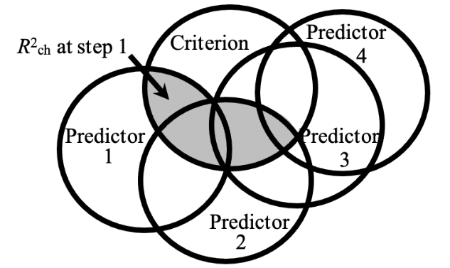
Unlike standard multiple regression, hierarchical multiple regression enters predictors in a pre-specified order. That is, the predictors get entered into the model in different “steps” or “blocks”. The model is assessed at each step, and the increment in explained variance (R2 change or R2ch) at each of these steps is usually the focus of interest.
At Step 1, we only enter the predictor(s) for Block 1 of the model (i.e., predictors 3 and 4 are not yet in the model). We assess the increase or change in the criterion variance (i.e., R2ch) that is explained by the entry of this first predictor or set of predictors into the model (in the case below, this is the set containing predictors 1 and 2). Therefore, R2ch at Step 1 would be represented by the shaded grey area in the diagram below.
Figure 5.5
Model at Step 1 Containing Only Predictors 1 and 2 (i.e., the First Predictor ‘Set’ or ‘Block’)
Then, at the next step, we add an extra predictor or set of predictors (in this case, our second set is made up of predictors 3 and 4). We again assess the change increment in the criterion variance (i.e., R2ch) that is explained at this second model step.
Figure 5.6
Model at Step 2 Containing Both Sets or Blocks of Predictors
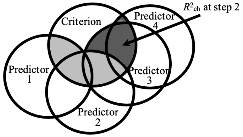
The dark shaded area (R2 change at Step 2) represents the proportion of variance explained by the second set of predictors (predictors 3 and 4) over and above the first set (predictors 1 and 2).
We also report the total amount of variance explained at the final step. In our example, this is R2 at Step 2. This would be calculated as the lighter shaded section (R2ch at Step 1) plus the darker shaded section (R2ch at Step 2) in Figure 5.6 above.
Exercise 2: Standard Multiple Regression
The Effects of Stress and Sex on Eating Difficulty (Again!)
In the simple regression/ correlation we performed in Exercise 1 in Activity 4, we worked with a clinical psychologist who was interested in eating difficulties. More specifically, the researcher was trying to examine the effects of stress on eating difficulty. This time, the researcher intends to explore the predictors of eating difficulty further. The researcher is aware that the kind of eating difficulties they are examining tend to occur in greater frequencies among females than males. Thus, they wish to add in the effects of biological sex as well as stress into their model to explain eating difficulty. To do this, the researcher has decided to get data from a larger sample. They expect that sex and stress as a combination will significantly predict eating difficulty (Hypothesis 1). Also, they believe that individually, both sex and stress will have unique contributions to the prediction of eating difficulty. Specifically, that (a) females will report experiencing more eating difficulties than males (Hypothesis 2a), (b) those with higher levels of stress will display more eating difficulty (Hypothesis 2b), and (c) sex will be a more important determinant of eating difficulties than stress (Hypothesis 2c).
Activity 5 Exercise 2 Part 1: Hypotheses for the Standard Multiple Regression
What analyses and statistical results match the researcher’s hypotheses?
Click to reveal the answer:
The answer is:
Hypothesis 1 refers to the overall standard multiple regression model with stress and sex (i.e., R2 will be significant). Hypotheses 2a and 2b refer to the unique contribution statistics for sex and stress, respectively (i.e., sr2/ b / β will be significant for each and in the anticipated direction as indicated by b/ β). Hypothesis 2c also refers to the unique contribution statistics for sex and stress, but looks to compare the absolute magnitude of these to see which is larger and therefore, more important as a predictor. This difference is assessed for significance using a Fisher's z test. While jamovi does not currently have this capability, we use information obtained in the output and through additional analysis (i.e., the partial correlation values) to determine this statistic via an online calculator. (NB: Don’t forget that the β, b, sr2 and pr2 for an individual predictor are all assessed with the same t-test. Hence use of the pr values for the Fisher's z test provides the same evaluation as to whether these unique predictor contributions differ significantly as would be given for β).
Part 2: jamovi for Standard Multiple Regression (SMR)
Next, we will look at how to run a standard multiple regression analysis, where multiple predictors are entered simultaneously into the model. The data for this exercise (an extension of the last data set on stress as a predictor of eating difficulty) have been entered for you in a file called “Multiple Regression Dataset”.
- Download the Multiple Regression Dataset (OMV, 3 KB), by going to the link and clicking the three dots and clicking download to download the file. Open the file after downloading by double clicking on the ‘.omv’ file if you have jamovi installed directly on your computer (or open jamovi and then open the file). Have a look at how the variables have been labelled and coded (especially for sex). NB, if it doesn't look like a data file in jamovi, you may have downloaded the metadata instead of the actual data, so please go back to the link above and click on the three dots next to the file name and then click download to try again.
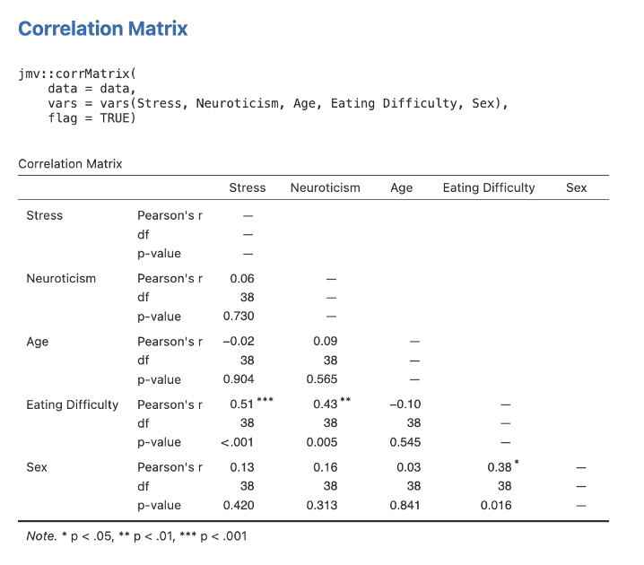
- We’ll start off by obtaining some scene-setting bivariate correlations. We do this by selecting Analyses -> Regression -> Correlation Matrix. Move all three variables (i.e., Eating Difficulty, Stress and Sex) into the righthand box for inclusion. Make sure Pearson is ticked in the Correlation Coefficients section on the far right. Under Additional Options tick the checkboxes next to Report significance and Flag significant correlations. Ensure that Correlated under Hypothesis is checked.
Figure 5.7
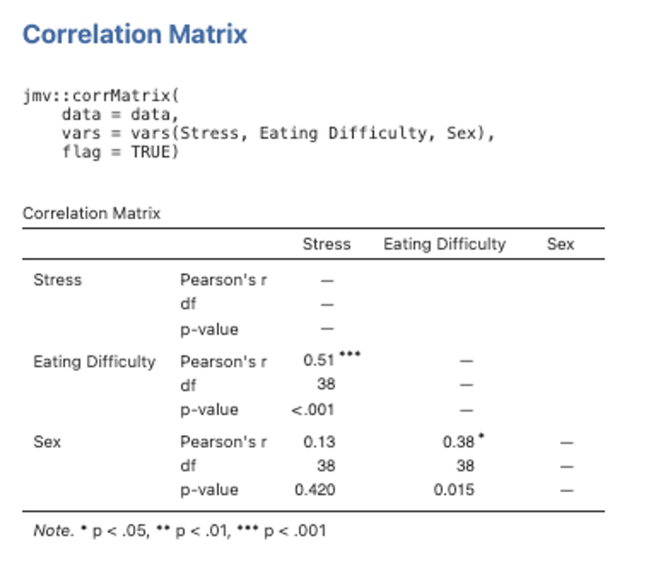
Note. A comment that can be made about the correlation table above is that the order has been determined by convenience (i.e., we simply moved all of our variables into the box without worrying about the order). This is fine when we just need the numbers for another table which we will be preparing in APA format. However, in your write-up, it is preferable to have the dependent measure as either the first variable listed or the last variable listed, with the IVs grouped together. So you may like to re-create the title putting Eating Difficulty (our DV) in as either the first or last variable, instead of in the middle as here!
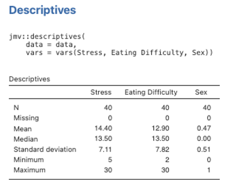
- We’ll also run some descriptives, so we have means and standard deviations for our variables to report alongside the bivariate correlations. Go to the Exploration menu on the Analyses menu ribbon and then select Descriptives. Move Eating Difficulty, Stress and Sex variables across to the right-side box.
Figure 5.8
- Now run the actual multiple regression analysis by selecting Analyses -> Regression -> Linear Regression. Select Eating Difficulty as the Dependent variable. Then select Stress as a Covariate (remember jamovi calls continuous independent variables covariates) and Sex as a Factor (remember jamovi calls categorical independent variables factors). Under the Model Fit dropdown menu we want to be sure we have R, R2 and Adjusted R2 selected, along with F test under the Overall Model Test. In the Model Coefficients drop down menu under the Standardized Estimate heading we want to select Standardized estimate and Confidence Interval (set to 95%).
Figure 5.9
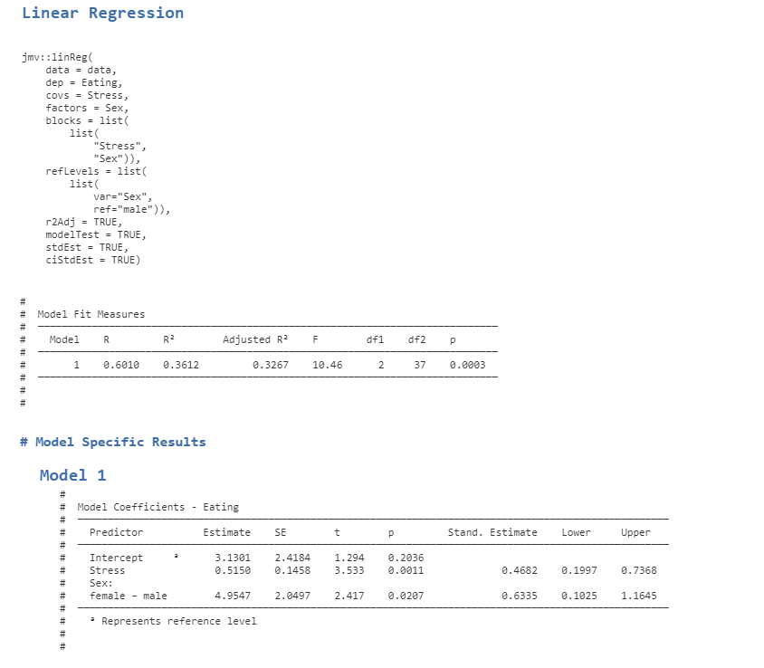
Note. To adjust the number of decimal places, access the settings menu in jamovi by clicking the three dots on the far right of the menu ribbon. You can separately adjust the decimal places for p values and other numbers. You can also toggle the syntax mode on and off so that the code is visible above the table of Model Fit results.
If we are reporting betas, we report them for each IV from the “Stand. Estimate” (i.e., standardised estimate) column, and the CIs for the betas are printed beside them to the right. If we wanted to report the unstandardised estimates (b), they are in the Estimate column, and we would need to run the analysis separately so that we get the appropriate unstandarised confidence intervals.
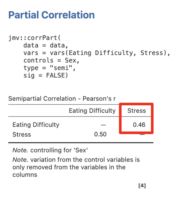
- In order to get our semi-partial correlations to report as effect size measures, we will have to run a separate analysis for each of our independent variables. We head back to the Regression menu on the Analyses tab ribbon. Then select Partial Correlation. Move Eating Difficulty and Stress into the Variables box and Sex into the Control Variables box. Under Correlation Type ask for Semipartial. Click underneath the results output just generated in order to allow jamovi to create a second set of output for this and not overwrite it. (To simplify your output, you can untick Report significance, as the p values are not needed in reporting the effect sizes.) The correlation value given under the column heading for the independent variable is the semi-partial correlation, highlighted in red. The correlation value given along the row of the independent variable is the bivariate correlation, which should match what we saw earlier in our descriptives analysis.
Figure 5.10
- Now go back to Partial Correlation and this time put Eating Difficulty and Sex into the Variables box and Stress into the Control Variables box. Again, ensure you have Semipartial selected under Correlation type.
Figure 5.11
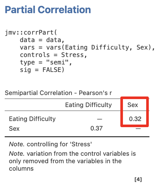
Here we see the sr for sex predicting eating difficulty, controlling for stress, is .32.
- When you've run both the analyses in steps 2 and 3, we will work systematically through how to perform the extra necessary calculations, as well as read, interpret and write-up these results. Pay particular attention to how you interpret the means, correlations and β values involving sex (which was dummy coded, i.e., coded as 0 and 1 for males and females, respectively).
Part 3: Work Out the Unique and Shared Variance Model Values
jamovi only supplies us with semi-partial correlation (sr) values. These need to be squared to obtain the necessary unique variance values for each predictor (i.e., sr2). Further, shared variance also needs to be determined for the model (i.e., R2 - Σsr2).
Stress:sr2stress = __________ = __________
Sex:sr2sex = __________ = __________
Shared variance: R2 - Σsr2 = R2 – (sr2stress + sr2sex) = ______________________________ = __________
Part 4: Determine the Fisher's z value to Assess if Predictors are Significantly Different in Their Strength of Prediction
Use an online calculator to determine the Fisher's z value and significance level between the pair of model predictors, e.g., Psychometrica.
This will determine whether or not the two predictors differed significantly in strength.
You will need to select “Comparison of correlations from dependent samples” (as we are comparing the strength of predictors within the same dataset, generated by the same participants). Then input information regarding the relevant:
- sample size (n),
- bivariate/ Pearson correlation between the criterion and first predictor of interest (r12),
- bivariate/ Pearson correlation between the criterion and second predictor of interest (r13), and
- bivariate/ Pearson correlation between the first and second predictors of interest (r23). This information can be found in the Correlations table.
Note that use of the bivariate correlations for this procedure only applies to a model with ONLY TWO predictors!
If we had more than two model predictors, we would replace r12 and r13 with the partial correlation (pr) values for the two predictors we were comparing. We would also need to calculate a separate partial correlation (pr) between the two predictors, controlling for the criterion and any other relevant predictors within the model (r23). This is achieved using the Partial correlation analysis function in the software.
NB: pay close attention that the pr values for the two correlations that you are comparing are both converted into POSITIVE values before you subsequently enter them into the online calculator (so you are comparing their absolute strength). If both are positive or both negative initially, enter the third correlation (r23) as is. If one of the two (r13 or r23) was negative and the other positive, when you enter the converted correlations as both positive, you should enter r23 as opposite in sign to what it was. So for example, if the correlations initially are -.2, -.4, .3 you would enter .2, .4, .3 (leaving r23 as it was because both r13 and r12 were negative). If the correlations are -.2, .4, .3 you would enter .2, .4, -.3 (converting r23 in sign).
Comparing Stress and Sex for a Significant Difference in Strength of Prediction:
Sample size (n) = _______r12 = _______r13 = _______r23 = _______
Fisher's z = __________p = __________
Part 5: Writing up the Results for a Standard Multiple Regression Analysis
- Describe the multiple regression analysis that was conducted, identifying the criterion and predictors. If this is the first time you have used the term “SMR” in the text, this acronym needs to be introduced properly, i.e., by writing "standard multiple regression (SMR)".
- Report the bivariate correlations between each predictor and the criterion (these are known as validities), as well as the intercorrelations between the predictors themselves (these are known as collinearities). State the significance/ non-significance of each, and provide the direction of effect. This is usually done in the text, with reference to a table that contains the means, standard deviations and bivariate correlation values for all the study variables. Be sure to provide an overall comment on (a) which predictors were valid vs. not valid within the model, and (b) whether collinearity was at a problematic level (i.e., if predictors overlapped too highly with one another, suggesting redundancy). NB: Because sex here is a dichotomous variable, you will need to describe the bivariate sex difference in eating difficulty, because a ‘positive’ or ‘negative’ correlation will not make sense (i.e., it could mean different things depending on how the coding was performed). So you will need to specify whether males/ females reported significantly higher eating difficulty levels than females/ males.
- Describe the analysis of regression. That is, describe the proportion of variance in eating difficulty that was explained by the predictors taken together (i.e., R2 expressed as a percentage in the text) and state the significance/ non-significance. Provide the statistical notation for the test of significance and significance level at the end of this sentence, i.e., F(df) and p. If confidence intervals (CI) were available for this whole model statistic, these could also be presented here (following the p-value notation).
- Now describe the unique contributions of the individual predictors, including their significance/ non-significance and direction. Reporting the relevant β, t(df), p, and 95% CI values associated with these. Also describe the proportion of variance in eating difficulty that can be explained uniquely by stress and sex (i.e., their sr2 values expressed as percentages in the text).
- State the amount of shared variability in the model (i.e., R2 - Σsr2, expressed as a percentage in the text). Also, comment on the order of importance of the predictors (base this on β weights or sr2 values and be sure to mention all predictors in the model). Evaluate predictor unique contributions for significant differences using Fisher's z test(s), stating significance/ non-significance, and order of strength. Provide the relevant statistical notation at the end of the sentence, i.e., z and p.
As a reminder:
- Values presented in a table should not be repeated in the text. Likewise, values given in a sentence should not be repeated as statistical notation (e.g., 36% of the eating difficulty variance…, R2 = .36). This is redundant reporting.
- Statistical notation in English/ Latin letters needs to be italicised (e.g., F, t, p, z), while that in Greek (e.g., β) appears as standard text. Likewise, notation for “95% CI”, as well as subscripts and superscripts are presented in standard text (i.e., these do not appear in italics).
- Inferential statistics (e.g., F, β, t, z), correlations (r) and confidence intervals should be presented to two decimal places, while p-values go to three. Since effect sizes (e.g., R2, sr2 and shared variance) will already be taken to two decimals before they are converted into a percentage (e.g., sr2 = .10 = 10%), these are left as whole numbers. Only in cases when the %s are all very low and need to be differentiated, do these get reported to two decimals.
- Descriptive statistics such as means and standard deviations are given to the number of decimals that reflect their precision of measurement. In our case, means and standard deviations should be taken to one decimal place for reporting.
- Values that can potentially exceed a threshold of ±1 (e.g., M, SD, F, t, z), should have a 0 preceding the decimal point. However, values that cannot potentially exceed ±1 (e.g., r, β, p, 95% CI for β), should not have a 0 before the decimal.
- The direction of effect for an individual predictor should also be reflected in the positive or negative valence of its reported β and t-value.
- Confidence intervals should span the β-value correctly. This means that a significant negative β will likewise have two negative CI values, a significant positive β will have two positive CI values, and a non-significant β-value (whether positive or negative) will have a negative lower bound CI value and a positive upper bound CI. In all cases, the β-value itself should be positioned directly in the middle of the reported CI value range (minus rounding considerations).
- When reporting confidence intervals, the % span for these is only stipulated the first time these are stated within a paragraph or single analysis e.g., 95% CI [lower, upper]. Following this, the percentage is not to be repeated, i.e., CI [lower, upper].
- Degrees of freedom (df) for an overall regression model are: (Regression df, Residual df), where these are found in the ANOVA output table. In contrast, df for a t-value are just: (Residual df), also found in the ANOVA table.
Part 6: Linking the Results Back to Predictions
Were the researcher’s predictions supported?
Exercise 3: Hierarchical Multiple Regression
The Effects of Sex, Age, Neuroticism and Stress on Eating Difficulty
Imagine now that the clinical psychologist has a slightly different focus in their research. This time, the main point of interest for them is to examine whether stress and neuroticism (a personality trait found to be positively linked to non-constructive coping strategies, such as disordered eating) will have a combined impact on eating difficulty after controlling for the effects of biological sex and age (a variable found to negatively predict eating difficulty in teenage and young adult populations). The researcher expects that, collectively, stress and neuroticism will still predict eating difficulty after the effects of age and sex have been controlled (Hypothesis 1). Further, they predict that – after controlling for age and sex – stress will be a more important predictor of eating difficulty than neuroticism (Hypothesis 2).
Activity 5 Exercise 3 Part 1: Hypotheses for the Hierarchical Multiple Regression
What analyses and statistical results match the researcher’s hypotheses?
Part 2: jamovi for Hierarchical Multiple Regression Analysis (HMR)
- You will need to have downloaded the data for Exercise 3, the Hierarchical Multiple Regression Dataset (OMV, 3 KB), by going to the link and then clicking on the three dots and clicking download. Double click the downloaded file to open it in jamovi, if jamovi is installed on your computer, or open jamovi and then open the file. Then, start by running scene setting bivariate correlations between all the variables. Head to Analyses -> Regression -> Correlation Matrix. Move all variables (i.e., Stress, Neuroticism, Age, Eating Difficulty, and Sex) into the box for inclusion.
- Make sure Pearson is ticked in the Correlation Coefficients section on the far right. Under Additional Options tick the checkboxes next to Report significance and Flag significant correlations. Ensure that Correlated under Hypothesis is checked. Given that we have not previously explored the variables of neuroticism and age with regard to eating difficulty levels, it is important that we conduct these correlations for this study (i.e., they are not redundant analyses in this case).
Figure 5.12
Note. If your output does not show the syntax, you are able to toggle this on by accessing the settings menu in jamovi (by clicking the three dots in the far right of the menu ribbon) and clicking syntax mode. Also, the correlation table above has the same issue raised previously regarding the order being determined by convenience. When preparing the table for your write-up, it is preferable to have the dependent measure as either the first variable listed or the last variable listed, with the IVs grouped together. For simplicity, therefore, as the tables get larger and more complex, it is worth spending a few seconds before running the software to choose a meaningful order. For example, put the DV first, then variables in Block 1, and variables in Block 2; or alternatively, put the IVs in the order entered, followed by the DV as the last variable.
We’ll also run some descriptives, so we have means and standard deviations for our variables to report alongside the bivariate correlations. Go to the Exploration menu on the Analyses menu ribbon and then select Descriptives. Move all variables across to the right-side box.
Figure 5.13
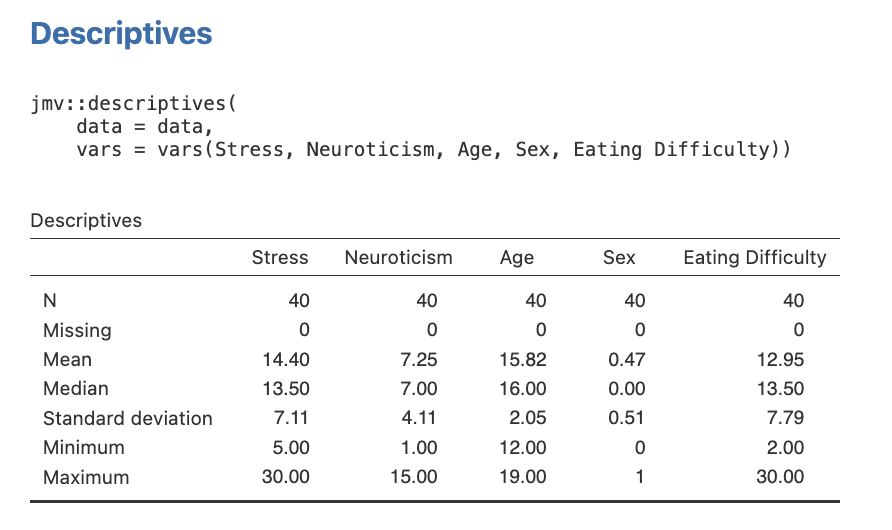
Note. You can change the number of decimal places displayed in your output for numbers and p values by accessing the settings menu (by clicking the three dots on the far right of the menu ribbon).
Answer to Part 1: a hierarchical multiple regression analysis would need to be performed on eating difficulty (criterion), with age and sex (predictors) entered into the model at Step 1, then stress and neuroticism (predictors) at Step 2. This analysis would address both hypotheses. For Hypothesis 1, if the amount of additional variance explained at Step 2 is significant (i.e., R2ch at Step 2 and the corresponding p-value), then this tells us that stress and neuroticism collectively predicted eating difficulty after controlling for the combined influence of age and sex. For Hypothesis 2, we would look to the magnitude of the β and/ or sr2 values for stress and neuroticism at Step 2 and assess these using a Fisher's z test to determine the more important predictor of eating difficulty. Specifically, the unique contribution for stress would need to be significantly larger than that for neuroticism to offer support for our second hypothesis (NB: note that this significance test is actually run using the partial correlation values for the predictors being compared).
- We will now run a hierarchical regression analysis where multiple predictors are entered into the model in a pre-specified order. We will control for age and sex at Step 1, and then add the second set/ block of predictors containing stress and neuroticism at Step 2.
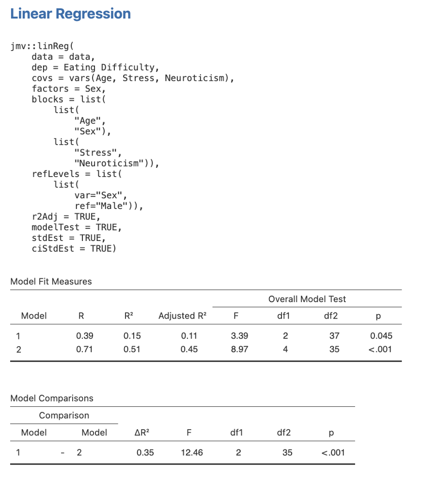
- Head to Analyses -> Regression -> Linear Regression. Select Eating Difficulty as the Dependent variable. Then select Age, Stress, and Neuroticism as a Covariates (remember jamovi calls continuous independent variables covariates) and Sex as a Factor (remember jamovi calls categorical independent variables factors). Under the Model Fit dropdown menu we want to be sure we have R, R2 and Adjusted R2 selected under Fit Measures and F test is selected under Overall Model Test. In the Model Coefficients under the Standardized Estimate heading we want to select Standardized estimate and Confidence Interval (set to 95%).
- The way we get our predictors into the steps we want them to be in is via the Model Builder dropdown menu. You’ll see that all four of our predictors are currently listed in Block 1. Move Stress and Neuroticism out of the Block 1 box by highlighting them and hitting the arrow pointing to the left. Under Blocks click Add New Block so that Block 2 appears. Now select Stress and Neuroticism and move them each across into the Block 2 section.
Figure 5.14
Note. If your output does not show the syntax, you can toggle this on by accessing the settings menu (by clicking on the three dots in the far right of the jamovi menu ribbon), where you can also change the decimal places.
Here is the first part of our output. In the Model Fit Measures table we have tests of the full model at each block/step (R2 and F). Model 1 includes the ANOVA for the inclusion of Age and Sex only. Model 2 includes the ANOVA for Age, Sex, AND Stress and Neuroticism – all four predictors.
In the Model Comparisons table jamovi provides a test of the increment in variance explained at each step (R2 change and F change). The test of R2 change is a test of whether Stress and Neuroticism (as a set/ block) added significantly to the prediction of eating difficulty over and above that of Age and Sex. Note that the test for R2 change is based on:
Figure 5.15
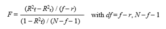
Text version of image:
[latex]F=\frac{(R^{2}_{f}-R^{2}_{r})/(f-r)}{(1-R^{2}_{f})/(N-f-1))}\:with\:df=f-r,N-f-1[/latex]
where f = the number of predictors in the full model (more predictors, in this case four),
and r = the number of predictors in the reduced model (fewer predictors, in this case two).
Note too that the increment in the criterion variance explained by stress and neuroticism as a set/ block at the last step of the hierarchical multiple regression (i.e., R2ch at Step 2) will often be lower than the value of R2 that would occur from a standard multiple regression analysis conducted with just stress and neuroticism. This is because the shared variance between each of these predictors and age and sex will have been absorbed by age and sex at Step 1 of the model. The only time it will be not be smaller is when predictors entered at later steps of the hierarchical multiple regression have no shared variance with those entered earlier in the model. If there's no overlap between the Step 1 and the Step 2 predictors (i.e., they are not correlated with each other), the R2ch at Step 2 will be the same as the R2 if you just ran a standard multiple regression predicting the DV from the variables entered at Step 2.
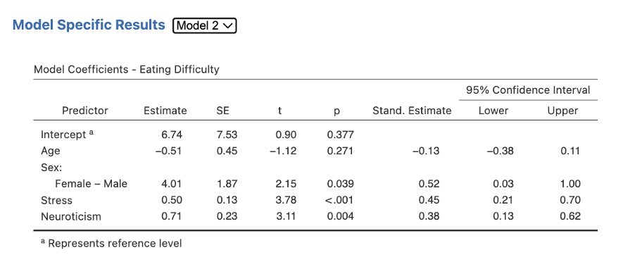
Depending on your version, to view the full results for our coefficients table for Step/Block 1 and Step/Block 2 you may have to toggle between views. Note how there is a drop-down list next to the Model Specific Results heading. Select Model 1, then select Model 2 to get all the sections of this table. Model 1 includes just the variables entered in Step 1 (Age and Sex). Model 2 now includes all four variables. In other versions of jamovi, Model 2 is reported right after Model 1, so you can see them both.
Figure 5.16
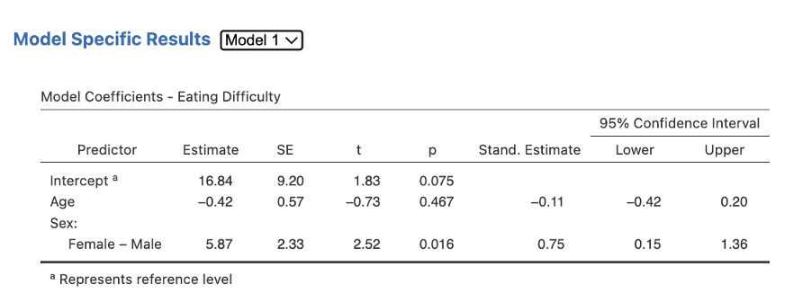
Figure 5.17
Note. To change the decimal places in your jamovi output, access the settings menu by clicking the three dots at the far right of the menu ribbon.
Finally, we need to obtain our semi-partial correlations. As jamovi can only provide these to us one at a time this is a little tedious, however we’ll go through each variable individually below which will make it more clear. Each time we will be heading back to the Regression menu on the Analyses tab ribbon, and then we will select Partial Correlation. We will move the DV and one IV at a time into the Variables box and the remaining predictors for that Step/Block/Model into the Control Variables box. (When calculating the partial correlations for Step 1, do not enter any Step 2 variables as control variables; only the Step 1 variables are considered in Step 1.) Under Correlation Type ask for Semipartial. The default option is that Report significance is ticked, and you may like to untick this as to report the effect sizes, we only need the semipartial correlation itself, not the p value.
Step 1 – Getting the Semi-Partial Correlations for Step/Model 1 for Age
Move Eating Difficulty and Age into the Variables box, and Sex into Control Variables.
Figure 5.18
Note. If you see the p values as well as the sr, you can turn this off by unticking Report significance in the options for the correlation analysis (or just ignore them - they are not needed to report our effect sizes). If you only see one correlation in your output instead of two, you likely have forgotten to ask for semipartial under correlation type.
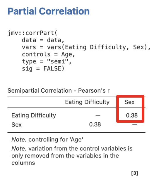
Step 2 – Getting the Semi-Partial Correlations for Step/Model 1 for Sex
Move Eating Difficulty and Sex into Variables, and Age into Control Variables.
Figure 5.19
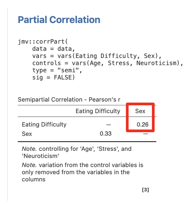
Step 3 – Getting the Semi-Partial Correlations for Step/Model 2 for Sex
Move Eating Difficulty and Sex into Variables, and Age, Stress, and Neuroticism into Control Variables.
Figure 5.20
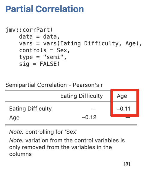
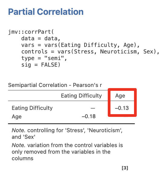
Step 4 – Getting the Semi-Partial Correlations for Step/Model 2 for Age
Move Eating Difficulty and Age into Variables, and Sex, Stress, and Neuroticism into Control Variables.
Figure 5.21
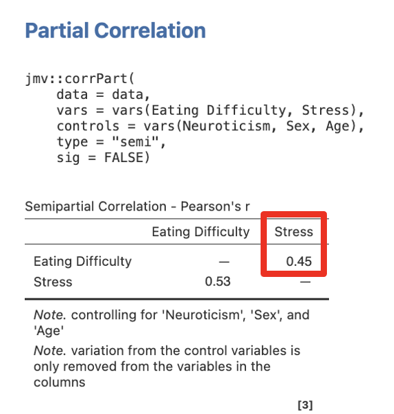
Step 5 – Getting the Semi-Partial Correlations for Step/Model 2 for Stress
Move Eating Difficulty and Stress into Variables, and Sex, Age, and Neuroticism into Control Variables.
Figure 5.23
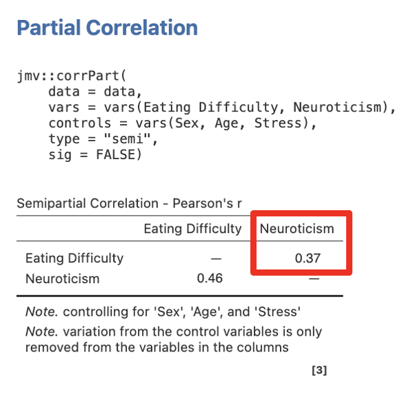
Step 6 – Getting the Semi-Partial Correlations for Step/Model 2 for Neuroticism
Move Eating Difficulty and Neuroticism into Variables, and Sex, Age, and Stress into Control Variables.
Figure 5.24
Part 3: Inspect the Output
When you understand all of the output, try to write up a Results section for it. A guide has been given to you for this below the output, so you may like to skip ahead to read the guide in Part 7 and then look through the output again.
Part 4: Work out the Unique and Shared Variance Model Values
Recall that jamovi only supplies us with semi-partial correlation (sr) values. These need to be squared to obtain the necessary unique variance values for each predictor (i.e., sr2) at the relevant model step, i.e., the block in which the predictor was entered. Further, shared variance also needs to be determined for each of the model steps (i.e., R2ch - Σsr2 for new predictors added to that model step).
Step 1:
Age: sr2age = __________ = __________
Sex:sr2sex = __________ = __________
Step 1 shared variance: R2ch at Step 1 - Σsr2 for new predictors added
= R2ch at Step 1 – (sr2age + sr2sex) = ______________________________
= __________
Step 2:
Stress:sr2stress = __________ = __________
Neuroticism:sr2neuroticism = __________ = __________
Step 2 shared variance: R2ch at Step 2 - Σsr2 for new predictors added
= R2ch at Step 2 – (sr2stress + sr2neuroticism) = ______________________________
= __________
Part 6: Calculate Fisher's z values to Assess if Predictor Strengths Differ Significantly
Use an online calculator to determine the Fisher's z value and significance level between the pair(s) of model predictors at each step, e.g., Psychometrica.
This will determine whether or not the predictors – entered at different model blocks for theoretical reasons – differed significantly in their strength of prediction. If there was some theoretical reason to compare all four predictors (e.g., if we had a hypothesis that spoke to this aspect or if we were conducting a standard multiple regression with these four predictors), then we would use the values from all four variables at the last model step and make comparisons between all. However, in our case, we were interested in their separate effects at the various model steps. Therefore, we will need to compare age and sex at Step 1, then stress and neuroticism at Step 2 (after controlling for the effects of age and sex).
Select “Comparison of correlations from dependent samples” (as we are comparing the strength of predictors within the same dataset, generated by the same participants). Then input information regarding the relevant:
- sample size (n),
- bivariate/ Pearson correlation between the criterion and first predictor of interest (r12),
- bivariate/ Pearson correlation between the criterion and second predictor of interest (r13), and
- bivariate/ Pearson correlation between the first and second predictors of interest (r23).
Given our model has MORE THAN TWO predictors, the values entered into the online calculator differ slightly and require extra jamovi analyses to gather relevant information!
Specifically, if we have more than two model predictors, we replace r12 and r13 with the partial correlation (pr) values for the two predictors we are comparing.
However, we also need to calculate a separate partial correlation (pr) between the two predictors (which will replace r23), controlling for any other variables at that model step (including the criterion). To get this we use the same Partial Correlation menu we used to get our semi-partial correlations. However, under Correlation Type you will ask for Partial not Semi-partial. For Step 1, move both Age and Sex (i.e., predictor 1 and predictor 2) into the Variables box, and Eating Difficulty (i.e., the criterion) into the Control Variables box.
Again, pay attention that the pr values for the two correlations that you are comparing are both converted into POSITIVE values before you subsequently enter them into the online calculator (so you are comparing their absolute strength). If both are positive or both negative initially, enter the third correlation (r23) as is. If one of the two (r13 or r23) was negative and the other positive, when you enter the converted correlations as both positive, you should enter r23 as opposite in sign to what it was. So for example, if the correlations initially are -.2, -.4, .3 you would enter .2, .4, .3 (leaving r23 as it was because both r13 and r12 were negative). If the correlations are -.2, .4, .3 you would enter .2, .4, -.3 (converting r23 in sign).
Comparing Age and Sex for Significant Difference in Strength at Step 1:
Sample size (n) = _______r12 = _______r13 = _______r23 = _______
Fisher's z = __________p = __________
NB: The partial correlation between age and sex (pr23.1 = r23 entered for this calculation) at Step 1 will only need to control for eating difficulty (the only other variable in the model).
Comparing Stress and Neuroticism for Significant Difference in Strength at Step 2:
Sample size (n) = _______r12 = _______r13 = _______r23 = _______
Fisher's z = __________p = __________
NB: The partial correlation between stress and neuroticism (pr45.123 = r23 entered for this calculation) at Step 2 will need to control for all the other variables in the model at Step 2, i.e., eating difficulty, age and sex.
Extra Exercise: Compare all four predictors at the last model step (i.e., Step 2).
Part 7: Writing up the Results for a Hierarchical Multiple Regression
Note. IF this was not our first analysis involving all four predictors of eating difficulty (i.e., age, sex, stress and neuroticism), then we would not need to perform point 2 below as this would be redundant reporting (i.e., these statistics would have been covered in earlier analyses). Yet whenever new predictors are included in the model (such as this case here regarding age and neuroticism), then the statistics within point 2 need to be presented.
- Describe the multiple regression analysis that was conducted, identifying the criterion and predictors. If this is the first time you have used the term “HMR” in the text, this acronym needs to be introduced properly, i.e., hierarchical multiple regression (HMR). Include the order of predictor entry into the model, and the rationale behind this order.
- Report preliminary analyses on the means, standard deviations, bivariate correlations between each predictor and the criterion (validities), as well as the intercorrelations between the predictors themselves (collinearities). State the significance/ non-significance of each correlation, and provide the direction of effect. As in Exercise 2, this is best done in the text, with reference to a table that contains the means, standard deviations and bivariate correlation values for all the study variables. Include overall comments on (a) which model predictors were valid/ non-valid, and (b) whether collinearity was an issue for the analysis model. NB: Because sex is a dichotomous variable, you will need to describe the bivariate sex difference in eating difficulty, because a ‘positive’ or ‘negative’ correlation will not make sense (i.e., it could mean different things depending on how the coding was performed for this variable). So you will need to specify whether males/ females reported significantly higher eating difficulty levels than females/ males.
- Describe the proportion of variance in eating difficulty that was explained by age and sex together at Step 1 (i.e., R2ch expressed as a percentage in the text). State whether this was significant/ non-significant, reporting the associated F change and significance level statistical notation at the end of the sentence, i.e., Fch(df) and p. As always, if confidence intervals (CI) were available for this model statistic, these would also be presented here (following the p notation).
- Describe the individual contributions of age and sex at Step 1. For each, specify the direction of effect and its significance/ non-significance. Report the appropriate statistical notation associated with each (i.e., β, t(df), p, and 95% CI). Provide the proportion of variance in eating difficulty that was explained uniquely by age and sex (i.e., sr2 for each, expressed as a percentage in the text). State the amount of shared variance present in the model at Step 1, expressed as a percentage in the text (calculated as: R2ch at Step 1 − sr2sex − sr2age). Also, comment on the order of predictor importance (based on the β weights or sr2 values). Evaluate these predictor strengths for a significant difference using a Fisher's z test, stating significance/ non-significance, and order of strength. Provide the relevant statistical notation at the end of the sentence, i.e., z and p.
- Describe the increase in R2 that results from the inclusion of stress and neuroticism as predictors at Step 2 over and above that explained by sex and age (i.e., R2ch expressed as a percentage in the text). Report whether this was a significant/ non-significant increment in R2, reporting the necessary F change and significance level statistics at the end of the sentence, i.e., Fch(df) and p.
- Describe the individual contributions of stress and neuroticism at Step 2. For both stress and neuroticism, state the direction of effect and significance/ non-significance. Provide the relevant statistical notation (i.e., β, t(df), p and 95% CI). Give the proportion of variance in eating difficulty that was uniquely explained by each of these new predictors (i.e., sr2 expressed as a percentage in the text for both). Present the shared variance for this model step, expressed as a percentage in the text (calculated as: R2ch at Step 2 − sr2stress − sr2neuroticism). Further, provide a statement comparing the importance of the stress and neuroticism predictors (based on their β and/ or sr2 values). Assess the difference in predictor strengths for significance using a Fisher's z test, stating significance/ non-significance, and order of strength. Be sure to include the associated notation at the end of the sentence, i.e., z and p.
- Lastly, describe the overall model at the final step. Specifically, report the proportion of variance in eating difficulty that was explained by age, sex, stress and neuroticism together (i.e., R2 at Step 2, as a percentage in the text). State whether this was significant/ non-significant, reporting the appropriate F(df) and p-value statistics. [This would be equivalent to the result obtained if we’d run a standard multiple regression analysis where all four predictors were entered simultaneously]. Once again, if confidence intervals (CI) were available for this whole model statistic, these could be given following the p-value notation.
As a reminder:
- Values presented in a table should not be repeated in the text. Likewise, values given in a sentence should not be repeated as statistical notation (e.g., 16% of the eating difficulty variance…, R2ch = .16). This is redundant reporting.
- Statistical notation in English/ Latin letters needs to be italicised (e.g., F, Fch, t, p, z), while that in Greek (e.g., β) appears as standard text. Likewise, notation for “95% CI”, as well as subscripts (e.g., “ch”) and superscripts are presented in standard text (i.e., these do not appear in italics).
- Inferential statistics (e.g., F, Fch, β, t, z), correlations (r) and confidence intervals should be presented to two decimal places, while p-values go to three. Since effect sizes (e.g., R2ch, R2, sr2 and shared variance) will already be taken to two decimals before they are converted into a percentage (e.g., sr2 = .15 = 15%), these are left as whole numbers. Only in cases when the %s are all very low and need to be differentiated, do these get reported to two decimals (and consistently so for all).
- Descriptive statistics such as means and standard deviations are given to the number of decimals that reflect their precision of measurement. In our case, means and standard deviations should be taken to one decimal place for reporting.
- Values that can potentially exceed a threshold of ±1 (e.g., M, SD, F, t, z), should have a 0 preceding the decimal point. However, values that cannot potentially exceed ±1 (e.g., r, β, p, 95% CI for β), should not have a 0 before the decimal.
- The direction of effect for an individual predictor should also be reflected in the positive or negative valence of its reported β and t-value.
- Confidence intervals should span the β-value correctly. This means that the β weight should be positioned directly in the middle of the reported CI value range (minus rounding considerations).
- When reporting confidence intervals, the % span is only stipulated the first time these are stated within a paragraph or single analysis e.g., 95% CI [lower, upper]. After this, the percentage is not to be repeated, i.e., CI [lower, upper].
- Degrees of freedom (df) for each model step are located under df1 and df2 of the Change Statistics in the Model Summary table (these represent Regression and Residual, respectively, for the change model at each step). In contrast, df for an overall regression model are: (Regression df, Residual df), which is found in the ANOVA output table at the final model step. Lastly, df for a t-value are just: (Residual df), but need to be found in the ANOVA table under the relevant model step.
Part 8: Linking the Results Back to the Hypotheses
Were the researcher’s hypotheses supported?
Test Your Understanding
- Explain the difference between squared partial and squared semi-partial correlations. What does each represent in terms of modelling the shared variance between variables? Use a diagram.
- Explain the difference between hierarchical and standard multiple regression.
- In analysing the relative importance of predictors, several kinds of statistics are useful, including the squared semi-partial correlation coefficient (sr2), the beta weight (β), and the bivariate correlation coefficient (r). Explain what each of these statistics measures, and how they differ from one another in terms of meaning.
- In which kinds of situations might a hierarchical multiple regression model be preferred over a standard one?
