
6 Activity 6 – Moderated Multiple Regression in jamovi
Last reviewed 19 December 2024. Current as at jamovi version 2.6.19.
Overview
In this section we examine how multiple regression analyses can be used to test for interactions among our (continuous) variables of interest. We learn how to examine the output to find the test of the interaction, and how to conduct follow-up analyses in the form of simple slopes for given levels of our variables in order to describe the nature of a significant interaction.
Learning Objectives
- To recognise the need for tests of interactions in multiple regression
- To understand the jamovi procedures for performing moderated multiple regression analyses
- To introduce the jamovi procedures for conducting simple slopes analysis to follow up a significant interaction
- To gain practice at writing up and presenting the results of a moderated multiple regression
Introduction to Moderated Multiple Regression
So far, we have treated multiple regression as being more or less analogous to the ANOVA models we have seen. That is, we have a number of predictor variables (or IVs) and we wish to use them to predict some of the variance in our criterion variable (or DV). However, as with ANOVA, another question of interest is whether the effects of one variable are consistent across levels of the other. In other words, do our variables interact?
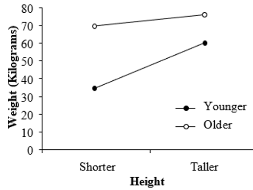
Consider the following hypothetical experiment. Let’s say we wanted to predict people’s weight and we had measurements on their height and age. A possible interaction that we could find might look like the graph below. Here, there is a strong positive relationship between height and weight for younger people, but only a weak relationship for older people. Therefore, age is moderating the effect of height on weight. Thus, we need to describe the two different slopes – one for older people, and one for younger people – in order to fully understand the nature of this relationship.
Figure 6.1
The Effect of Height on Weight as Moderated by Age
Consider what this means in terms of the variance we are trying to model in our criterion variable. We have already explained a certain amount of variance in weight (criterion) based on the combined scores of height and age. Yet we can explain a little bit more if we also include the interaction in our model. This interactive effect – represented by the product of the person’s height (in cm) and age (in years), which results in a new score (height*age) – adds explanatory power to our weight prediction equation.
Simple Slopes Analysis
Just as we tested the simple effects in ANOVA in order to understand an interaction, we need to test the simple slopes in multiple regression (the effect of one variable, at different levels of the other variable). Simple slopes analysis in regression is like simple effects analysis in ANOVA, but in multiple regression we are often working with continuous variables which have a potentially infinite number of scores that could be observed. Hence, we choose levels of one variable (e.g., “older” and “younger”) in order to graph the relationship, and to test the significance of the slopes (βs) of the other variable (e.g., height) at each of these levels.
By convention, the arbitrary levels we choose for low and high groups for each variable are 1 standard deviation from the mean. So, for the “Younger” analysis (i.e., the simple slope of height for younger participants – seen in the bottom line of the graph above), we would consider participants who score -1SD on age. For the “Older” analysis (i.e., the simple slope of height for older participants – seen in the top line of the graph above), we would consider an age score of +1SD. Similarly, for the height variable, we could separate out two values of “Taller” and “Shorter” by considering scores of +1SD and -1SD on height, respectively. We will illustrate how these calculations are performed later in this section.
Activity 6 Exercise 4: Moderated Multiple Regression
The Effects of Stress and Self-Esteem on Eating Difficulty
The psychologist studying eating difficulties has a new hypothesis. While they still believe that people who tend to report high levels of stress tend to have more eating difficulty, there could be a buffer to this effect. From what they have noticed clinically, people who have high self-esteem do not seem to show this association between stress and eating difficulty. That is, it doesn’t seem to matter how stressed a person with high self-esteem gets, this person’s eating difficulty level will not change. The researcher would like to test this observation quantitatively. They collect data from 40 psychology students. The students complete the same 10-item stress scale (total score range: 0-40), and 14-item eating difficulty scale (total score range: 0-42). However, they also complete a single item self-esteem question, which is measured on a 4-point scale (range 1-4, with higher scores indicating higher self-esteem). The researcher predicts that:
-
- Stress and self-esteem, when considered together, will predict scores on eating difficulty.
- A Stress x Self-Esteem interaction will be found. Specifically, they predict that when self-esteem is low, the positive relationship between stress and eating difficulty will be present. However, when self-esteem is high, there will be no relationship between stress and eating difficulty.
Part 1: Hypotheses for the Moderated Multiple Regression
What analyses and statistical results could be used to answer each hypothesis?
There are a couple of ways we could answer the first hypothesis. We could run a standard multiple regression, with stress and self-esteem entered simultaneously. A test on R2 of that model would answer Hypothesis 1. However, because Hypothesis 2 asks about an interaction (and hence, a moderated multiple regression is needed to address this), it would be easier to answer Hypothesis 1 using the information gathered at Step 1 of a moderated multiple regression. That way, we would only need to perform one analysis, rather than two. Besides being more parsimonious, this would also minimise our Type I error rate. So, at Step 1 of the moderated multiple regression, we will assess the combined direct effects of stress and self-esteem, by looking at the result for R2 change at Step 1 (which is assessed for significance using an F change test, which also provides a significance level, i.e., p-value).
Okay, now for Hypothesis 2. We are looking at an interaction here. So we will need to use a moderated multiple regression analysis. More specifically, we will need to enter the additive model at Step 1 (i.e., the regression equivalent of “main effects”, which are known as “direct effects”). Then, the interaction needs to be added into the model at Step 2. The interaction could then be examined by looking at R2 change at Step 2 (which is again assessed with an F change test, which gives rise to its significance level, i.e., p-value). However, this would only tell us that an interaction existed. To describe the actual nature of that interaction, we would need to follow it up with simple slopes analysis. Now, given the wording of the hypothesis, it seems that we want the simple slopes of STRESS (at each level of self-esteem). That is, our prediction is about how stress (key predictor) affects eating difficulty (criterion), and we want to separate that effect out for a high and low level of self-esteem (moderator).
Part 2: jamovi for Moderated Multiple Regression (MMR)
Data for this exercise (examining the effects of self-esteem and stress as predictors of eating difficulty) have been entered for you in a file called “Moderated Multiple Regression Dataset”. To test if stress and self-esteem interact to predict eating difficulty, we compute the cross-product of the two predictors (to create our interaction term), and then enter it into a hierarchical multiple regression analysis after entering the two direct effects. But first, we centre the continuous predictors around their respective means before computing the interaction term. This minimises multicollinearity between the original direct predictors and the new interaction variable.
- Download the Moderated Multiple Regression datase (OMV, 3 KB), by going to the link and clicking on the three dots next to the name and then clicking Download. From your computer, open this file up (by double clicking on the ‘.omv’ file if you have jamovi installed directly on your computer, or by starting jamovi and then opening the file). Have a look at how the variables have been labelled.
- To create the new mean-centered variable for stress, which we will label Stress Centered, go to the Data tab and click on Compute. In the Variable Name box type in Stress Centered. You will see a formula box with an = in it ready for you to create a formula to compute this variable. Click on the small box next to it with the fx in it. This will bring up a list of functions and a list of variables. We want to create a formula which is the Stress variable minus its mean (so for each participant in our data set we want to calculate their score minus the mean of the stress variable). Find Stress in the Variables list and double click on it. This will make it appear in the formula box. Then type in a – (dash) to act as a subtraction sign. Next in the Functions section scroll to find VMEAN (which stands for variable mean) and double click it. You will now get VMEAN( ) appearing with the cursor appearing in the parentheses. Double click on Stress again in the Variables list and you should now have a formula that reads “Stress – VMEAN(Stress)”. Click out of the formula set up and you should see the variable appear in the data set with values in it.
- Repeat the above process but for the Self Esteem variable. You’ll want to create a variable called Self Esteem Centered using the formula Self Esteem – VMEAN(Self Esteem).
- Finally to compute the interaction variable, select to Compute another new variable. However, this time in the formula box create the formula “Stress Centered * Self Esteem Centered”.
You are now ready to run the moderated multiple regression model.
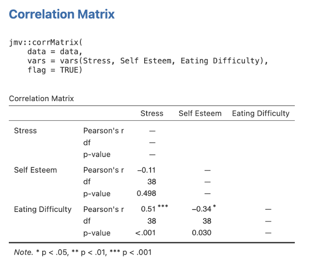
- Firstly we’ll ask for our scene setting bivariate correlations. Go to the Analyses tab and from the menu ribbon select Regression then Correlation Matrix. Select our original three variables (Stress, Self Esteem, and Eating Difficulty and click on the arrow button to move these into the right-hand box for inclusion in the analysis. Make sure Pearson is ticked in the Correlation Coefficients section on the far right. Under Additional Options tick the checkboxes next to Report significance and Flag significant correlations. Ensure that Correlated under Hypothesis is checked as this will give us a two-tailed significance test
Figure 6.2
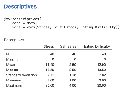
- Next we need some means and standard deviations for our variables for reporting purposes. Head to the Exploration menu on the Analyses menu ribbon and then select Descriptives. Move the Stress, Self Esteem, and Eating Difficulty variables across to the right side box. The default descriptives options here will give us what we need (mainly the means and standard deviations). The table will look like the one below.
Figure 6.3
- Run a moderated multiple regression. Head to Analyses Regression Linear Regression. Select Eating Difficulty as the Dependent variable. Then select Stress Centered, Self Esteem Centered and Centered Interaction and move them to the Covariates box (remember jamovi calls continuous independent variables covariates).Under the Model Fit dropdown menu we want to be sure we have R, R2 and Adjusted R2 selected under Fit Measures and F test is selected under Overall Model Test. In the Model Coefficients under the Standardized Estimate heading we want to select Standardized estimate and Confidence Interval (set to 95%).
- We need to enter our Centered Interaction variable into Step/Block 2 of our regression. So like we did for the hierarchical multiple regression we need to go to the Model Builder dropdown menu. You’ll see that our three predictors are currently listed in Block 1. Move Centered Interaction out of the Block 1 box by highlighting it and hitting the arrow pointing to the left. Under Blocks click Add New Block so that Block 2 appears. Now select Centered Interaction and move them each across into the Block 2 section.
Figure 6.4
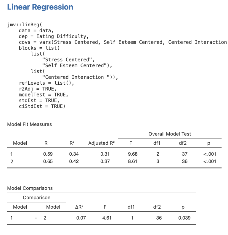
Here is the first part of our output. In the Model Fit Measures table in Figure 6.4, above, we have tests of the full model at each block/step (R2 and F). Model 1 includes the ANOVA for the centered versions of Stress and Self Esteem only. Model 2 includes the ANOVA for the two centered predictors as well as the interaction term.
In the Model Comparisons table in Figure 6.4, above, we see a test of the increment in variance explained at each step (R2 change and F change). The test of R2 change is a test of whether the interaction term added significantly to the prediction of Eating Difficulty over and above the direct/main effects of Stress and Self Esteem. R2 change in the Model Comparisons table is reported as delta R2 (so in Figure 6.4, R2 change = ΔR2 = .07).
Remember from covering Hierarchical Multiple Regression in Activity 5 that to view the full results for our coefficients table for Step/Block 1 and Step/Block 2 we have to toggle between views. Note how there is a drop down list next to the Model Specific Results heading. Select Model 1, then select Model 2 to get all the sections of this table.
Figure 6.5
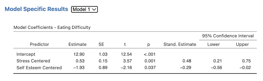
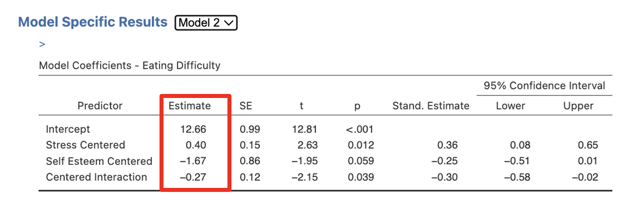
When you look at the Model 2 results, note that these four numbers will be required later on to graph the interaction using the Excel Simple Slopes file described below.
Figure 6.6
Finally, we need to obtain our semi-partial correlations. Each time we will head back to the Regression menu on the Analyses tab ribbon. Then select Partial Correlation. Move Eating Difficulty and each predictor in turn into the Variables box and the remaining predictors for that Step/Block/Model in Control Variables box. Under Correlation Type ask for Semipartial.
Step 1 – Getting the Semi-Partial Correlations for Step/Model 1 for Stress Centered
Move Eating Difficulty and Stress Centered to Variables, and Self Esteem Centered into Control Variables.
Figure 6.7
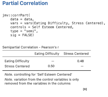
Take note of the confusing reporting: the semi-partial is reported in the columns (here, sr = .48) and the bivariate correlation is reported in the rows (so r = .50).
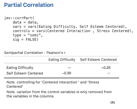
Step 2 – Getting the Semi-Partial Correlations for Step/Model 1 for Self Esteem Centered
Move Eating Difficulty and Self Esteem Centered to Variables, and Stress Centered into Control Variables.
Figure 6.8
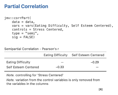
Again, be careful to pick out the relevant sr = -.29 (the correlation on the right) and ignore the bivariate correlation which is confusingly reported as well.
Step 3 – Getting the semi-partial correlations for Step/Model 2 for Self Esteem Centered
Move Eating Difficulty and Self Esteem Centered to Variables, and Stress Centered and Centered Interaction into Control Variables.
Figure 6.9
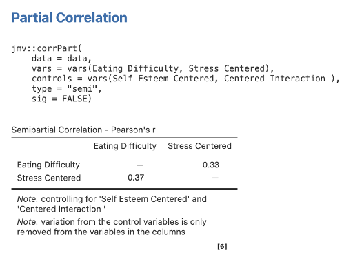
Step 4 – Getting the Semi-Partial Correlations for Step/Model 2 for Stress Centered
Move Eating Difficulty and Stress Centered to Variables, and Self Esteem Centered and Centered Interaction into Control Variables.
Figure 6.10
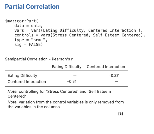
Step 4 – Getting the Semi-Partial Correlations for Step/Model 2 for Centered Interaction
Move Eating Difficulty and Centered Interaction to Variables, and Self Esteem Centered and Stress Centered into Control Variables.
Figure 6.11
Part 3: Inspect the Output
While we have shown you above how to calculate the sr2 for centered stress and centered self-efficacy in either block, for your write-up of the moderated multiple regression, in the text you would report the sr2 for the direct effects of the IVs from Step 1 only. However, we often need to add the sr2 for Step 2 because we are including a table with the full statistics for the analyses. Just check carefully what you are being asked for to avoid mistakes. For Part 4, when asked about Step 1, you will use the info in Figure 6.7 and 6.8.
Part 4: Work out the Unique and Shared Variance Model Values
jamovi only provides semi-partial correlation (sr) values. These need to be squared to give the necessary unique variance values for each predictor (i.e., sr2). Further, shared variance also needs to be determined for each model step as relevant (i.e., R2ch – Σsr2 for new predictors added to that model step).
Step 1:
Stress:sr2stress = __________ = __________
Self-Esteem:sr2self-esteem = __________ = __________
Step 1 shared variance: R2ch at Step 1 – Σsr2 for new predictors added
= R2ch at Step 1 – (sr2stress + sr2self-esteem) = ______________________________ = __________
Step 2: Some extra notes about MMR Reporting
sr2: Given that only one new predictor (i.e., the interaction) was added at Step 2, we do not need to calculate nor report the sr2 value for this interaction predictor. This is because it is equivalent to the R2ch value we provide at Step 2 and therefore, would represent redundant reporting. You can, however, check that you get the same % for both (i.e., R2ch at Step 2 = sr2interaction).
Shared variance: Note that no shared variance at Step 2 needs to be determined. This is because only one new predictor (i.e., the interaction) was added to the model at this step. Shared variance between the variables within a step only exists – and thus only needs to be calculated – when more than one predictor is added at a model step.
Exercise 5: Conducting Simple Slope Analyses in jamovi
You have now determined that a significant interaction exists in the data. Your next job is to describe it. For this you will need to perform “simple slopes analysis”, which are the regression equivalent of simple effects in ANOVA. Because we don’t have categorical (i.e., group) variables, this is a little harder. We have to create “categories”, which by convention, are one low (-1SD below the mean) and one high value (+1SD above the mean) on our moderator variable. Recall that back when we looked at our hypotheses, we determined that self-esteem was our moderating variable.
Simple slopes are not available to us within the Regression menu we have used so far. We will need to use an additional jamovi module called gamlj (General analysis for linear models in jamovi).
Click on + Modules on the far right of the menu ribbon then select jamovi library
- Within the jamovi library search for gamlj and click to install it. You should now have a “Linear Models” menu appearing in your Analyses ribbon.
- Select Linear Models then General Linear Model.
- Move the dependent variable (i.e., Eating Difficulties) into the Dependent Variable box. Move Stress and Self Esteem (in their original raw form) into the Covariates box (remembering this is what jamovi calls continuous predictors)
- Under Effect Size ensure the η2 and β checkboxes are ticked. Untick partial η2. Under Confidence Intervals ensure that Confidence Intervals is ticked (leave as 95%).
- In the Model dropdown box highlight both predictors in the Components box and arrow them across into the Model Terms box. This should now have both predictors plus an interaction term.
- In the Covariates Scaling dropdown box ensure that both predictors are set to Centered. Covariates conditioning should have Mean + SD selected and Dependent variable scale should be set to None (in other words, jamovi will use the original scale for the DV and will not change it).
- In the plots dropdown box select Stress and move it to the Horizontal axis box and Self Esteem to the Separate lines box. In Display leave it as None, and set Plot to display Y-axis observed range (this rescales the Y axis).
- In the simple effects dropdown box move Stress to Simple effects variable and Self Esteem to Moderator variable.
Head to the Simple Effects section of the output.
Figure 6.12
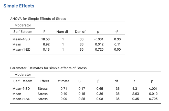
Note. Your output also will have the confidence intervals ticked to appear. To change the decimal places, access the settings menu by clicking the three dots in the far right of the menu ribbon.
Also examine the Simple Slopes Plot.
Figure 6.13
Note. If your x-axis is centered (showing -10 to 10 for the stress variable instead of the real range) you can go back to Covariates scaling and change Stress to None. The pattern will not change in the graph, but the labelling of the x-axis will be uncentered. Note that you should change the scaling for Stress back to Centered after checking the corrected x-axis. Depending on the version, there may also be a setting you can toggle under Plots for “Use original x-axis”. This is a small bug that I am sure they will fix in later versions of jamovi, but it’s not super critical to get your jamovi graph axes right as we are going to redo the graphs in Excel anyways in Exercise 6 so that we can implement APA formatting.
Exercise 6: Plotting the SIMPLE SLOPES
At this point, we have identified that there is a significant two-way interaction between stress and self-esteem. We have also discovered that the effect of stress on eating difficulty is significant when self-esteem is low, but non-significant when self-esteem is high.
What we would like to do now is create a line graph (like the ones you have done previously in factorial ANOVA) to show the effect of stress on eating difficulty at each level of self-esteem.
We will be using an Excel Macro to do this. We can’t use the one that is output from jamovi in our papers, assignments, and honours theses because it is missing APA 7 formatting. However, we can use the jamovi graph to get a sense of what our Excel graph will look like.
Before we get into this Excel graphing, however, we must remind ourselves of some key relevant information from our study design and jamovi output that we will need to enter into this program. Specifically, take note of the variable names:
Key predictor (IV): __________ Moderator: __________ Criterion (DV): __________
Also note the unstandardised coefficients (from the estimates column) of the original analysis (i.e., not the simple slope analyses):
Unstandardised coefficient (b) for constant: __________
Unstandardised coefficient (b) for key predictor (IV): __________
Unstandardised coefficient (b) for moderator: __________
Unstandardised coefficient (b) for interaction: __________
Standard deviation (SD) for moderator: __________
Standard deviation (SD) for key predictor (IV): __________
Standard error (SE) for low simple slope: __________
Standard error (SE) for high simple slope: __________
NB: You will not need to track down the means for your variables, as these were mean-centred remember? This means that the means for your key predictor (IV) and moderator will both be 0.
- Now download the Excel Macro for Simple Slopes (XLSX, 38 KB) and double-click on it. Before working in this document, Save As an Excel file with a name of your choosing.
- You will notice three tabs at the bottom left of this Excel file, each representing a different spreadsheet. The first reads “Two-Ways”, the second is “Three-Ways” and the third is a blank worksheet. You need to select the tab for Two-Ways so that you can create a graph of your two-way interaction.
- You will see that there are several sections on the Excel file that are coloured orange/ apricot. Wherever you see this colour, you will need to enter data from the exercise activity we completed (you should have entered this key information into the box above for easy reference).
- You will also see that there are several sections on the Excel file that are coloured green. These values will be created by Excel, based on the information you give it. DO NOT type anything in these green cells!
- In cell E5, you need to type in the name of the moderating variable (mod). So type Self-Esteem in this cell.
- In cell E6, you need to type in the name of the key predictor (iv). Type Stress in this cell.
- In cell M27, you need to type the name of the criterion (DV). Type Eating Difficulty in here.
- In cells F4 – F7, you are required to type in the unstandardised b weights for the final step in the moderated multiple regression analysis (see the output from Exercise 4). Be careful here – do not confuse this output with that from either of the simple slopes analyses. Further, be aware that the order in which the output provides these numbers is often not the same as we require them. Always check that the correct value matches up with the correct variable!
- In cell F4, type in the b weight for the constant. This is 12.661.
- In cell F5, type in the b weight for the moderator (Self-Esteem). This is -1.674.
- In cell F6, type in the b weight for the key predictor (Stress). This is 0.401.
- In cell F7, type in the b weight for the interaction term. This is –0.266.
NB: If you are wondering why we enter the unstandardised regression coefficient (b) values here to create the graph (rather than β weights), one reason is that we want to display the interaction and its constituent simple slopes on the original criterion scaling, as this is more intuitive for your reader to view and understand. In our case, this was the 0-42 scaling used to measure participants’ eating difficulty level in the study.
- In cells C10 – C11 you need to type in the means for the moderator and the predictor. As we have mean-centred each of these variables, this part is easy.
- In cell C10, type in the mean-centred mean for Self-Esteem. This is 0.
- In cell C11, type in the mean-centred mean for Stress. This is also 0.
- In cells D10 – D11 you need to type in the standard deviations for the moderator and the predictor.
- In cell D10, type in the standard deviation for the moderator (Self-Esteem). Recall that this comes from your Descriptives output). This value is 1.17670.
- In cell D11, type in the standard deviation for the key predictor (Stress). Again, this comes from your jamovi MMR output in the Descriptives table. This value is 7.11012.
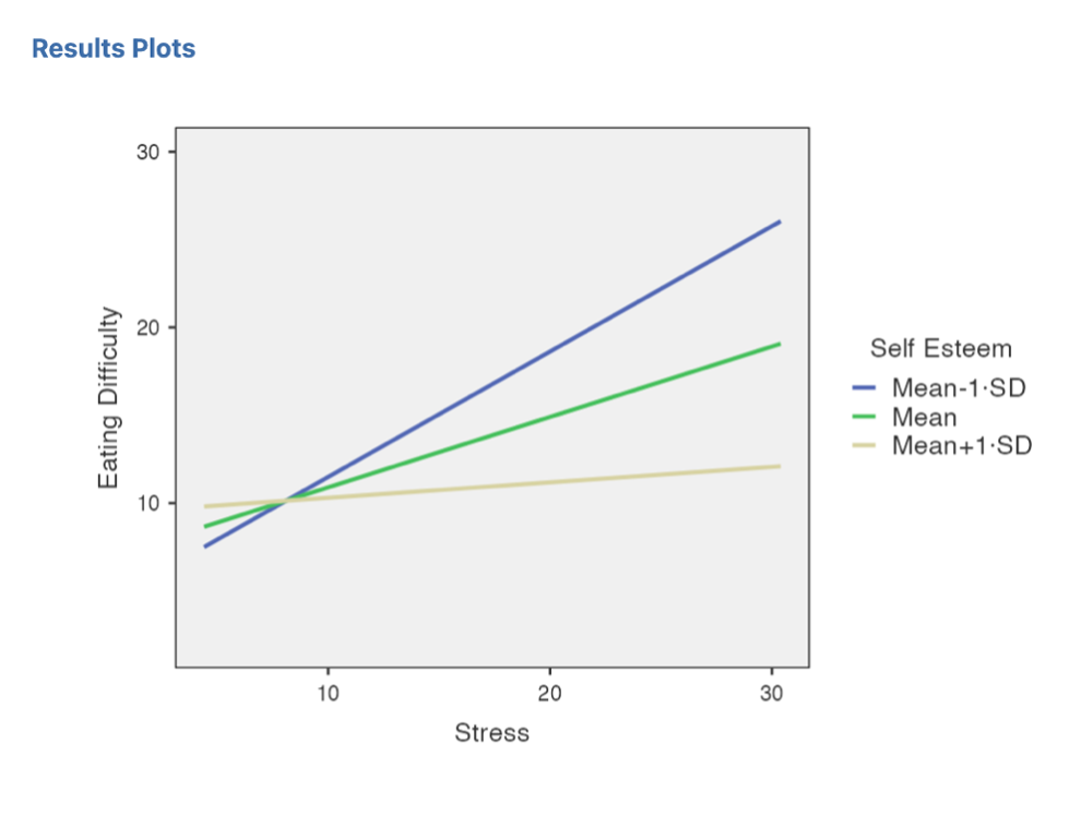
The figure that is shown to the right of the spreadsheet is the one that you want, i.e., you want the graph with the key predictor (stress) on the x-axis, and separate lines for the moderator (self-esteem). In its raw form, it should look like this:
Figure 6.14
This graph shows the predicted scores on eating difficulty as a function of stress and self-esteem. Low and high values are those which fall one standard deviation below and above the mean, respectively. Note. While this graph is close to proper APA format, there are still a few key aspects missing. So you will have to “tweak” it a bit by (1) labelling the x and y-axes, (2) adding error bars, (3) potentially changing the y-axis scores (to accommodate error bars as necessary), and (4) including a suitable figure title above and relevant notes below the figure (see Format Expectations workbook for instructions on this).
A Quick Guide:
- Axes titles/ labels can be achieved using text boxes. Remember to present these centred over their axis, with bold 12-point Times New Roman or 11-point Arial font (where the font style should match the rest of the document text).
- Error bars need to be added manually – one set for each simple slope. Click on one simple slope, and click on the “+” sign that appears to the right of the graph. Move down and click on the arrow next to Error Bars and select More options. Ensure that Both is chosen as the Direction and Cap as the End Style for your error bars. Then under Error Amount, click Fixed value and enter the standard error value for that simple slope in the box. Hit Enter and close the Format Error Bars box. Repeat this process for the other simple slope with its associated standard error value.
- The y-axis title should specify the full range of criterion/ DV scaling if this is not used, e.g., “Eating Difficulty (0-42)”. (Another approach is that you can simply label the y-axis “Eating Difficulty” and add a note under the table: “Note. Eating difficulty ranged from 0 to 42.”). There may also be times when the y-axis scaling has to be extended to accommodate the error bars in full. Simply right-click on the y-axis of the graph in Excel, select Format Axis and change the values for the Minimum and Maximum bounds as needed.
- The figure title (positioned above) and notes (positioned below) for a figure are best entered in the Word document itself, after the figure has been copy-and-pasted in. Take note of the use of bold, italics, title case letters (i.e., capitals for major words) and double-spacing within the title section. The notes below need to detail what low and high values were conceptualised as, what the error bars represent and if error bars happen to be small, they need to flag that they are difficult to see but are still present. For example:
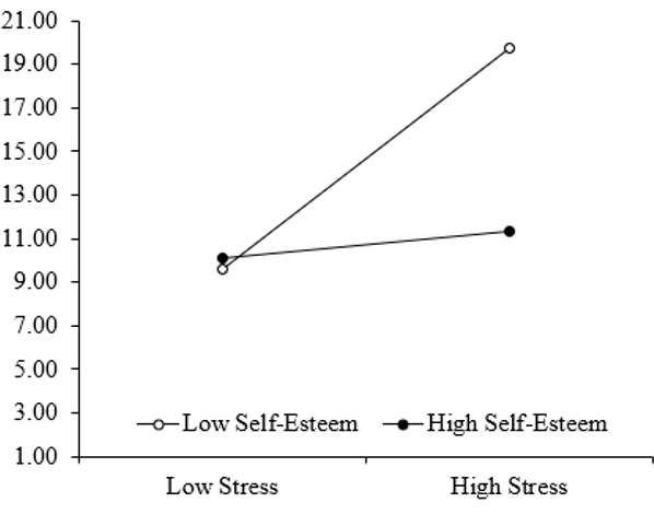
Figure 6.15
The Predicted Effect of Stress on Eating Difficulty Scores as Moderated by Self-Esteem
Note. Low and high values represent one standard deviation below and above the mean, respectively, for each variable. Error bars represent ±1 standard error (±1SE) from the mean, though values are too small to be seen easily on this graph.
Alternative Plotting of Simple Slopes (OPTIONAL)
You can also plot the simple slopes by doing a series of hand calculations. The steps are outlined below.
Write the unstandardised regression equation from the interactive model which used MEAN-CENTRED scores (i.e., what you calculated in Exercise 4).
To make it a little easier to read, let’s call the mean-centred self-esteem (cSE) variable “ESTEEM” and the mean-centred stress (cStress) variable “STRESS”.
= _______STRESS + ________ESTEEM + _______Interaction + _______
Remember that the interaction term = STRESS*ESTEEM, so re–write the above on the next line (but this time “Interaction” is now called “STRESS*ESTEEM”).
= ________STRESS + ________ESTEEM + _______STRESS*ESTEEM + _______
Now rearrange the equation to express the relationship between stress and eating difficulty as a function of stress.
= ( ________ + ________ESTEEM ) STRESS + (________ESTEEM + ________)
Solve this equation for the two values of self-esteem, so that you have an equation for each line (i.e., at ±1SD on ESTEEM).
High self-esteem (+1SD above the mean. Remember to use the mean-centred SE!) =_____
(Where do I find the standard deviation for self–esteem? Go to the Descriptive Statistics table in your output from Exercise 4. Remember that the mean is now zero because we have mean-centred our variables.)
= (_______ + ________ * _______) STRESS + (_______ * _______ + _______)
= ________ STRESS + _________
NB: You could also get this equation from the b weights for cStress and the constant in Step 2 of the moderated multiple regression/ simple slope where you used the “highSE” variable, i.e., Part 2 from Exercise 5.
Low self-esteem (–1SD below the mean. Remember to use the mean-centred SE!) = _____
= (_______ + ________ * _______) STRESS + (_______ * _______ + _______)
= ________ STRESS + __________
NB: You could also get this equation from the b weights for cStress and the constant in Step 2 of the moderated multiple regression/ simple slope where you used the “lowSE” variable, i.e., Part 1 from Exercise 5.
To plot the two simple slopes (for low self-esteem and high self-esteem), we need to find two points on each line (at ±1SD on stress).
The value for high stress (+1SD above the mean. Remember to use the mean-centred stress!) = ________
The value for low stress (–1SD below the mean. Remember to use the mean-centred stress!) = ________
Now substitute in each stress value (high and low), in turn, into the high self-esteem equation:
1. High stress & high self-esteem: = 0.088 (________) + 10.691 =
2. Low stress & high self-esteem: = 0.088 (________) + 10.691 =
These two numbers will be your data points when you plot the line for “high self-esteem”.
Now substitute in each stress value (high and low), in turn, into the low self-esteem equation:
3. High stress & low self-esteem: = 0.713 (________) + 14.631 =
4. Low stress & low self-esteem: = 0.713 (________) + 14.631 =
These two numbers will be your data points when you plot the line for “low self-esteem”.
Now calculate the significance of each slope, by conducting a t-test. The formula for t is:
The t-test uses N-p-1 degrees of freedom, where:
N is the total sample size, and
p is the number of predictors in the model at Step 2 (including the interaction term).
Calculate the following t-tests (one for each slope), keeping in mind that the critical t for 36 df (α = .05) = ±2.0281.
Low self-esteem slope:
= _______ = ________ so this result is: sig. / non-sig.
High self-esteem slope:
= _______ = ________ so this result is: sig. / non-sig.
Now plot the simple slopes with stress on the x–axis.
The moderator (self-esteem) will have separate lines, and eating difficulty will be on the y-axis! You also need to add error bars, using the appropriate simple slope SEb value for the two points on each line (above and below each point to make a 2SE span in total). NB: If these error bars are too small to be viewed clearly on the graph, you need to add to the note below that this is the case (e.g., see Figure 5 note above).
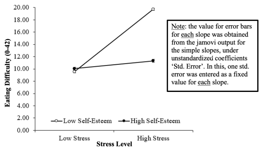
Figure 6.16
The Predicted Effect of Stress on Eating Difficulty Scores as Moderated by Self-Esteem

Note. High and low values were calculated as one standard deviation above and below the mean, respectively, for each variable. Error bars represent ±1 standard error (±1SE) from the mean.
Exercise 7: Writing up the Results of a Moderated Multiple Regression
If you have reported the results of another analysis prior to this that described the relevant preliminary analyses on the variable means, standard deviations, and zero-order correlations (e.g., in a standard multiple regression), then you would not repeat these in your moderated multiple regression write up as this would be redundant reporting (i.e., these statistics and results would have been covered in earlier analyses). However, if this has not been done, then you would report these after point 1 below, prior to the model Step 1 statistics. Look back to the write up sections for the SMR and HMR for what this should cover.
Describe and Explain the Analysis
Report the type of multiple regression analysis that was performed (i.e., a moderated multiple regression analysis), identifying the criterion and predictors. Remember, the interaction term is a predictor too. If this is the first time you have used the term “MMR” in the text, this acronym needs to be introduced properly, i.e., moderated multiple regression (MMR). Note which variables were mean-centred and WHY this was done. State how the interaction term was calculated. Then describe the order of entry of predictors into the model, and the rationale behind this order, i.e., to determine whether the interaction of stress and self-esteem explained additional variance in eating difficulty OVER AND ABOVE that of the direct effects (additive model) of these variables.
Report Step 1 Statistics:
Describe the proportion of variance in eating difficulty that was explained by the combined direct effects of stress and self-esteem at Step 1 (i.e., R2ch at Step 1 expressed as a percentage in the text). State whether this was significant/ non-significant, reporting the associated F change and significance level statistical notation at the end of the sentence, i.e., Fch(df) and p. As always, if confidence intervals (CI) were available for this change model statistic, these could also be presented here (following the p notation).
Go on to describe the individual contributions of stress and self-esteem at this step. Specify the direction of effect and significance/ non-significance for each of these predictors. Report the relevant associated statistical notation for each, i.e., β, t(df), p, and 95% CI. Give the proportion of variance in eating difficulty that each explained uniquely (i.e., sr2 for each, expressed as a percentage in the text). Also state the amount of shared variance present in the model at Step 1, expressed as a percentage in the text (calculated as: R2ch at Step 1 – sr2stress – sr2self-esteem).
Report Step 2 Change Statistics:
Report the increase in R2 that results from the inclusion of the interaction term in the model at Step 2 over and above that explained by the direct effects of stress and self-esteem (i.e., R2ch at Step 2 expressed as a percentage in the text). State whether this was a significant/ non-significant increment in the explanation of eating difficulty variance, reporting the appropriate F change and significance level statistics at the end of the sentence, i.e., Fch(df) and p. Again, if confidence intervals (CI) were available for this change model statistic, these could be presented following the p notation.
Report whether this indicated there was a significant/ non-significant interaction present, giving the appropriate statistical notation, i.e., β, t(df), p and 95% CI. Note that we do not state the direction of effect for this in the text, as it does not really make sense to talk about the interaction being a ‘positive’ or ‘negative’ predictor. Further, we do not provide the sr2 value for the interaction at Step 2 (either as notation or as a percentage in the text), as this is redundant reporting, i.e., sr2interaction = R2ch at Step 2.
Report the Overall Model at Step 2:
Report the total proportion of variance in the criterion (eating difficulty) that was accounted for by the two direct predictors AND the interaction at Step 2 (i.e., R2 at Step 2, as a percentage in the text). State whether this overall model was significant/ non-significant, reporting the corresponding significance test statistics, i.e., F(df) and p. [This would be equivalent to the result obtained if we’d run a standard multiple regression analysis where all three predictors were entered simultaneously]. Once again, if confidence intervals (CI) were available for this whole model statistic, these could be given following the p-value notation.
Report the Follow-Up Tests of the Interaction:
If there is a significant interaction, display this in a figure (be sure to have separate lines representing the moderator variable) and reference this figure in the text. Explain that the significant interaction was followed up by performing simple slopes analysis. NB: if the interaction had not been significant, we would not follow this up with simple slopes analysis!
Explain that values one standard deviation above and below the mean were used as high and low values, respectively, for each variable.
- Describe the effect of stress on eating difficulty when self-esteem was low. Report whether it was significant/ non-significant and state the direction of effect. Include the corresponding statistical notation at the end of the sentence i.e., β, t(df), p, 95% CI and sr2. Note that the latter effect size value appears as notation rather than as a percentage in the text for the simple slope reporting.
- Describe the effect of stress on eating difficulty when self-esteem was high. Describe whether it was significant/ non-significant, stating the direction of effect. Report the appropriate notation to accompany this, i.e., β, t(df), p, 95% CI and sr2. Again, we report the effect size value as statistical notation (i.e., sr2) rather than as a percentage in the text for this.
As a reminder:
- Values presented in a table should not be repeated in the text. Likewise, values given in a sentence should not be repeated as statistical notation (e.g., 34% of the eating difficulty variance…, R2ch = .34). This is redundant reporting.
- Statistical notation in English/ Latin letters needs to be italicised (e.g., F, Fch, t, p), while that in Greek (e.g., β) appears as standard text. Likewise, notation for “95% CI”, as well as subscripts (e.g., “ch”) and superscripts are presented in standard text (i.e., these do not appear in italics).
- Inferential statistics (e.g., F, Fch, β, t), correlations (r) and confidence intervals should be presented to two decimal places, while p-values go to three. Since effect sizes (e.g., R2ch, R2, sr2 and shared variance) will already be taken to two decimals before they are converted into a percentage (e.g., sr2 = .03 = 3%), these are left as whole numbers. Only in cases when the %s are all very low and need to be differentiated, do these get reported to two decimals (and consistently so for all).
- Descriptive statistics such as means and standard deviations are given to the number of decimals that reflect their precision of measurement. In our case, means and standard deviations should be taken to one decimal place for reporting.
- Values that can potentially exceed a threshold of ±1 (e.g., M, SD, F, t), should have a 0 preceding the decimal point. However, values that cannot potentially exceed ±1 (e.g., r, β, p, 95% CI for β), should not have a 0 before the decimal.
- The direction of effect for an individual predictor should also be reflected in the positive or negative valence of its reported β and t-value. Note that even though we do not talk about the interaction being a ‘positive’ or ‘negative’ predictor, it will still be reported with the relevant sign in front of its associated statistics.
- Confidence intervals should span the β-value correctly. This means that the β weight should be positioned directly in the middle of the reported CI value range (minus rounding considerations).
- When reporting confidence intervals, the % span is only stipulated the first time these are stated within a paragraph or single analysis e.g., 95% CI [lower, upper]. After this, the percentage is not to be repeated, i.e., CI [lower, upper].
- Degrees of freedom (df) for each model step are located under df1 and df2 of the Change Statistics in the Model Summary table (these represent Regression and Residual, respectively, for the change model at each step). In contrast, df for an overall regression model are: (Regression df, Residual df), which is found in the ANOVA output table at the final model step. Lastly, df for a t-value are just: (Residual df), but need to be found in the ANOVA table under the relevant model step.
- sr2 for simple slopes is typically given as notation. This is presented as a proportion (i.e., sr2 = .23, not sr2 = 23%) following the CIs. If this value is ever very small (i.e., would round to .00 or 0%), it gets reported as sr2 < .01.
Recommended Extra Readings
Note that it is also possible to calculate moderated multiple regression using standardised scores instead of mean-centred scores. For a discussion of this, see Cohen et al. (2003). Applied multiple regression/ correlation analysis for behavioural sciences (Chapter 7). Lawrence Erlbaum.
The book section below deals with the limitations of regression analyses, theoretical issues and the minimum required ratio of cases-to-predictors to run multiple regressions effectively:
Tabachnick, B. G., & Fidell. L. S. (2018). Using multivariate statistics (7th ed., Chapter 5, pp. 121-127). Pearson.
Test Your Understanding
- Explain why the inclusion of the interaction term in an analysis may increase the power of our model in explaining the variance in the criterion.
- Consider a few examples of psychological constructs that might have continuous predictors (e.g., intelligence, anxiety level). See if you can think of interactive – as well as additive – models that could explain each variable.
