
7 Activity 7 – Conducting Within-Participants (aka Repeated Measures) ANOVA using jamovi
Last reviewed 21 February 2025. Current as at jamovi version 2.6.19.
Overview
In this section, we look at how within-participants (aka ‘repeated measures’) ANOVA can be conducted using jamovi.
We look more closely at how we can check the data to make sure that it meets the assumption of sphericity, and we introduce a way of adjusting the degrees of freedom to make our test more conservative in response to violations of this assumption. Finally, we look at designs involving more than one within-participants variable, as an extension of the one-way case.
Learning Objectives
- Recognise and be familiar with the jamovi procedures for conducting within-participants (repeated measures) ANOVA, including follow-up tests and interpretation of the associated jamovi output
- Identify and understand the statistics for testing sphericity, and the methods of adjustment that are used in cases where there are violations of this assumption
- Extend the conceptual formulae of the within-participants ANOVA to study designs involving more than one within-participants variable
Understanding Within-Participants (Repeated Measures) ANOVA
Recall that the logic of the between groups ANOVA involved separating out the variance in the DV into two sources of variance – between-groups variance, and within-groups variance. While the between-groups design specified that participants only are associated with one of the levels of each independent variable, another kind of research design we might use employs the same people in every condition of an IV. This is referred to as a “within-participants” (or “repeated measures”) design. In within-participants ANOVA, variance is partitioned in a different way to between-groups designs to establish the effects of our factors.
Consider the case with only one within-participants factor of interest. We are interested in the effect of time of day (morning, midday, or night time) on reaction times. The experimenter gathers observations for each person at each level of the independent variable (i.e., every participant does the reaction time task three times: in the morning, at midday, and at night time). So, the differences between observations reflect two sources of variance: between-participants variance (i.e., differences between people on the measure: some people are faster), and within-participants variance (i.e., differences between observations within the same person: a person could be faster at a particular time of day).
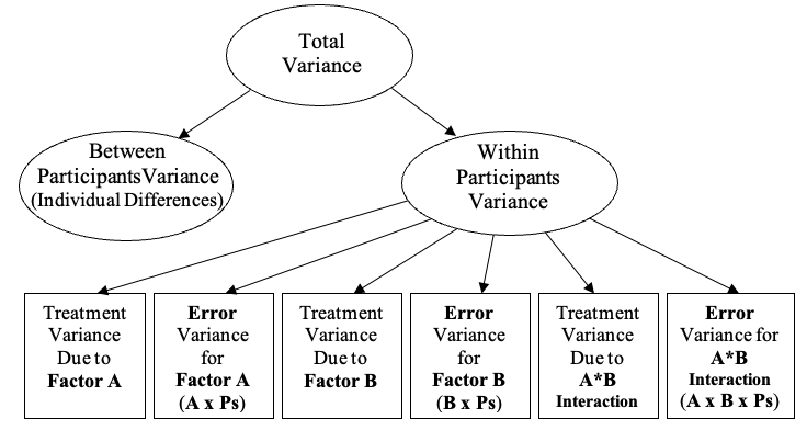
Figure 7.1
Partitioning of Variance in a One-Way Within-Participants (Repeated Measures) ANOVA
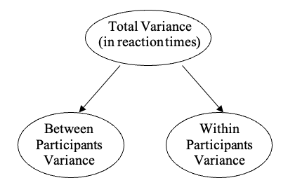
When we have repeated measurements for the same participants, we can calculate a main effect for the differences between participants. This effect is like a control variable in our analysis: we don’t always report it, but include it in the design to reduce Type 2 error. That is, instead of treating individual differences as error (which we have done in the between groups ANOVA), individual differences are now a separate factor in our analysis. Because individual differences are separate, the error term will always be smaller in a within-participants study design compared to a between groups design. Put differently, because we remove individual differences from the error term (and measure them as a factor), the power of any test for the focal IV in a within-participants study will always be greater than the test of the same IV in a study that uses a between-groups design with the same scores and the same sample size, when error is bigger because individual differences are not controlled.
So in a within-participants design, the total variability in observations includes the average differences between individuals (the individual differences control factor), as well as the second factor, our focal variable of interest: the differences between the observations for different levels of the independent variable. In the one-way within participants ANOVA, this is our treatment effect.
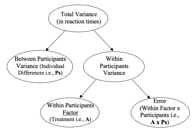
Since we have accounted for individual differences (which we are factoring out, like a control variable), and we have also accounted for differences between levels of the independent variable (our focal IV), what then does our error term represent in the within-participants design? Our error is going to be the interaction between the individual differences factor and the effects of the within-participants factor, our focal IV or treatment variable. The interaction conceptually measures how the effects of the within-participants factor change differently depending on the individual: one person might show slower reaction time as the day gets on from morning to noon to night, while another person speeds up over the course of the day. So, this interaction is the error term in a within-participants design, and it represents the inconsistency of the effect of the focal IV on the DV, times of day on reaction times, for the different individuals. In a one-way design with Factor A as our repeated measures variable, the error term is often written as “AxPs” or “AxP”, meaning the interaction between the within-participants factor (A) and participants’ individual differences (Ps).
Consequently, the variance in the one-way within participants design looks like this:
Figure 7.2
Partitioning the Within Participants Variance in a One-Way Within Participants (Repeated Measures) ANOVA
Assumptions of Within-Participants ANOVA
If you recall, one of the basic assumptions of between groups ANOVA is that the observations in each condition are independent. That is, an observation in one condition in an experiment should not depend on any other observation. Obviously, when you measure the same individual several times, this assumption no longer holds, because a person’s score when measured the first time is related to their score when measured the second time, because of the individual differences factor (P).
Instead, we make a substitute assumption for within-participants ANOVA, which is known as the assumption of sphericity. Effectively, the assumption of sphericity means that scores for any two conditions should correlated similarly to scores for any other pair of conditions. We will now look at how to test this assumption, and what to do when the assumption is violated (which it often is).
The Sphericity Test
Conducting within-participants ANOVA in jamovi allows us to specifically test our sphericity assumption, by examining the variances and covariances of the measures. Essentially, this examines the degree to which the measurements correlate with one another, to ensure that these are roughly equal. The test used is the Mauchly Sphericity Test (or Mauchly’s W).
When sphericity is violated, some of the conditions or levels of the IV are more closely correlated than other levels are. For example, the first and second levels of the within-participants factor may be more highly correlated than the first and third levels are. Unadjusted F tests show Type 1 error when sphericity has been violated, i.e., they have false positive results and alpha > .05. One option researchers have then is to ignore the ANOVA, and to perform a multivariate test such as a MANOVA, which does not require sphericity, but has its own concerns not addressed in this chapter. A better option is to adjust to make the test more conservative, which is what researchers generally prefer to do.
Essentially, adjusting an F test for violations of sphericity is done by adjusting the degrees of freedom associated with the test by a fixed amount, called an epsilon adjustment. The epsilon ranges from 0 to 1 and the smaller it is, the lower the degrees of freedom. For example, if the epsilon is 0.5, and the original degrees of freedom for the F test in our one-way design were (2, 98), the revised degrees of freedom after the epsilon adjustment become 1, 49 (multiplying each degree of freedom by 0.5). Lower degrees of freedom makes the critical test of the results more conservative, so that the error rate after adjustment returns to alpha = .05 and there is no inflated Type 1 error.
Jamovi outputs two possible adjustment values for each F-ratio, which represent two commonly used epsilon formulae. Disconcertingly, the p values for the tests of our focal IV will change based on which epsilon we pick, so it is best to adopt a strategy ahead of time as to which we will employ, instead of just picking based on which results we like the best! As a general rule, we recommend reporting the Greenhouse-Geisser epsilona, since it makes an adjustment to the degrees of freedom proportional to the violation of sphericity that has occurred in the empirical data. It is, therefore, neither too lax nor too conservative.
a It may seem odd to talk about statistics using words like “generally recommended”. Unfortunately, it is one of those facts of life that things are never as clear cut as we would like. There are many fuzzy decisions that need to be made in analysing data, and the further you go in statistics, the more complicated these decisions become.
Exercise 1: One-Way Within-Participants (Repeated Measures) ANOVA in jamovi
Leisure activity preferences
An enthusiastic tutor in PSYC3010 believed that her students were really enjoying their statistics study, so much so, that they were enjoying study more than other leisure activities! To test this hypothesis, five students from PSYC3010 were randomly selected and asked to complete a pencil-and-paper questionnaire that required them to rate the satisfaction they gained from various leisure activities. The activities included reading, dancing, watching TV, studying statistics, and skiing. The Likert-type rating scale used for these items ranged from 0 (no satisfaction at all) to 10 (extreme satisfaction). The tutor expects that:
- There will be differences in overall satisfaction gained from these various leisure activities, and
- Students will find studying statistics more satisfying than watching TV.
1. What statistical effects/results would match each hypothesis?
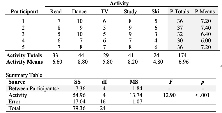
2. Here is the raw data and summary table for this exercise
Table 7.1
Raw Data and ANOVA Summary Table for One-Way Within-Participants ANOVA
Go to a version of Table 7.1 formatted for accessibility.
b This line and test are normally omitted, as we only focus on the within-participants factor of theoretical interest. But just FYI, the between-participants (i.e., individual differences) statistics are taken from the error values for the between participants effect below. The MS 1.84 in the “Tests of Between-Subjects Effects” table (see later output) measures variation of individuals around the sample’s mean score. Larger variance means that people are more different from each other (which is a fundamental part/ definition of being an individual). In this case all participants are scoring between 6.00 and 7.40 on a scale from 0 to 10, so they are relatively similar to each other in their average enjoyment across all activities, and the variance is small. We could compare the SS between Ps to the total SS (7.36/79.36) and observe that 9% of the variability in activity ratings is accounted for by individual differences, averaging across activities. We could test this against the error term for Activity, in theory, but we have only five participants, and it is not good to use this design and such a small sample if individual differences are a theoretical focus (because whichever five participants you pick could change the between-Ps result markedly). You would use a different design and probably worry about seeking representative sampling if you wanted to get a meaningful estimate of individual differences in the population.
Step 1: Enter the Data
- You need 5 columns to enter the data for each participant. The first column will be used to indicate the participant’s motivation score for the first activity. The next four columns will be used to represent the other four levels of the within-participants factor activity type. Working in an active jamovi window, click on the Variables tab in the analysis ribbon to define your variables. Type in the first variable name (i.e., Read) in row A. In the Setup box, define the measure type as Continuous.
- Type in the variable names Dance, TV, Study, and Ski in the rows underneath Read in the Variable view.
- Click on the Data tab in the analysis ribbon to enter the data. You will see that the five variables you created are now the five columns of the dataset. In the within-participants design, there will be one column to enter the scores for participants for every level of the within-participants factor. You will also need 5 lines in total (one line for each participant).
- Be sure to save your data to a suitable place under an appropriate name.
Alternatively you can download the jamovi file (Block 3 Activity 7 Exercise 1 – One way Within ANOVA.omv; 12kb) with the data entered already for you. After clicking through the link, click on the three dots next to the name and then click Download. From your computer, open this file up (by double clicking on the ‘.omv’ file if you have jamovi installed directly on your computer, or by starting jamovi and then opening the file). After you have downloaded the file, have a careful look at how the variables have been labelled.
Step 2: jamovi for within-participants ANOVA
- Type in or open your relevant dataset. Inspect the data.
- Select Analyses -> ANOVA -> Repeated Measures ANOVA … to open the Repeated Measures ANOVA analysis options.
- In the Repeated Measures Factors box, type in the name of your within-participants factor (i.e., Activity) in the RM Factor 1 heading. In each level provided underneath type in the name of each of the activities in turn. Note you can click add to add more levels until you have added all five levels in.
- In the Repeated Measures Cells box drag each variable from the left hand column into its respective slot that has been created from Step 3.
- Under Effect Size tick the box.
- Under the Assumption Checks drop down menu, select Sphericity tests, and select Greenhouse-Geisser as well as Huynh-Feldt along with None under Sphericity corrections. Huynh-Feldt epsilon is another common episilon adjustment which we introduce here so you can compare the results. Note that a) we recommend always reporting Greenhouse-Geisser epsilon adjusted F tests, and b) you should pick your epsilon in advance and not change your decision based on what the results show.
- Finally in order to obtain means and standard deviations, head to the Exploration menu on the Analyses ribbon, click on Descriptives and then select and drag all five variables across into the right hand Variables box to obtain descriptive statistics for reporting.
Step 3: Examine the output
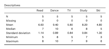
Consider the descriptives obtained in Step 7 first:
Figure 7.3
Descriptives for Activity Types in jamovi
We mentioned earlier that there is another way of handling within-participants designs: the multivariate approach. The way that we are using here is called a mixed-model approach, and it is the common way of analysing within-participants designs. The term ‘mixed-model’ reflects the fact that we have one or more fixed factors (Activity) and a random factor (participants). That is, our model is a mix of fixed and random factors. Fixed factors are those where you select the levels in advance (i.e., we chose which five activities we would study when we were designing the study). Random factors are those where you take whatever levels you find (e.g., the participants who end up in the study are random, not selected by us during the design phase).
In the present chapter, we are focusing on understanding the mixed-model output. Other statistical software such as SPSS will provide output for both the multivariate and mixed-model approaches, however jamovi just provides the mixed-model approach output which is what most researchers report.
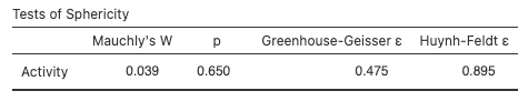
Let’s direct our attention to Mauchly’s Test of Sphericity, which checks that we have not violated the assumption of sphericity. In this case, the statistic is not significant, indicating that we could assume sphericity is present if we wanted. However, the Mauchly’s test is not very robust, so we recommend to inspect the epsilon values provided regardless of what the test shows.
The Greenhouse-Geisser epsilon provides an epsilon adjustment which is proportional to the magnitude of departure from sphericity in the data. The Huynh-Feldt epsilon is an adjustment of the Greenhouse-Geisser epsilon which we asked for for comparison: you will see that the p value for the test of the focal IV reported when you use the Huynh-Feldt episilon is lower than the p value of the test reported with the Greenhouse-Geisser epsilon, making the focal IV look more significant. There’s another extremely conservative epsilon adjustment (the lower-bound epsilon) reported by some software packages, like SPSS, but few scholars use that one because it’s seen as being prone to Type 2 error (false negatives).
Note: The sphericity assumption only applies when there are THREE or more levels of the repeated measures IV. Where there are only two levels jamovi will report a Mauchly’s W and epsilon values of 1 and an NaN error in the p column with a footnote stating the assumption of sphericity is automatically met when only two levels are present. However, sometimes this NaN error appears with epsilon values of 1 as an error when you have three or more levels of a repeated measures IV as a result of issues with the variance formula. If this happens you will have no choice but to report unadjusted F results, as no corrected results will be provided. In this instance it will be important for you to acknowledge the result is not epsilon-adjusted and may have a Type I error bias when discussing findings in the discussion of a research report.
Figure 7.4
Test of Sphericity in jamovi
After the sphericity test, we get the test of the within-participants effects (called by its outdated name “within-subjects”). We only have the one within-participants factor, i.e., Activity. Note that the test is provided three times, each with a different adjustment to the degrees of freedom.
Figure 7.5
Within-Subjects Effects in jamovi
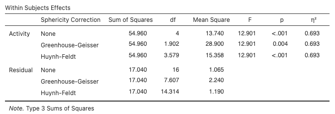
Indicate for each test whether or not this is a statistically significant result:
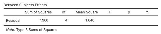
Next, we see the tests of between-subjects effects (labelled by its outdated name “between-subjects”). What we reported earlier in our summary table is the variance due to participants’ individual differences (MS 0.94). This is considered ‘Error’ or AKA ‘Residual’ in this table because it is being used automatically to test whether the overall mean for participants (“Intercept”) is different from zero. It usually is in psychology, which is not surprising especially because we often use scales that do not include zero (e.g., 1 to 7 or 1 to 10). Beyond measurement issues, however, the existence of individual difference variability is generally taken for granted by psychologists, and this is another reason the test of the individual differences factor is not usually reported. Like all software, jamovi output often contains things that we ignore.
Figure 7.6
Between Subjects Effects in jamovi
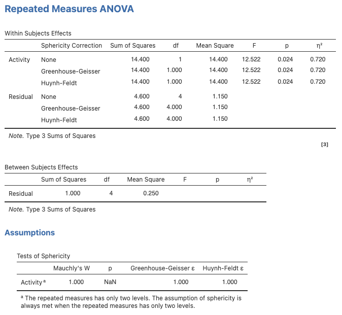
Step 4: jamovi for main effect comparisons in a within-participants factorial design (following up a significant main effect)
Since our within-participants factor (the focal IV) is significant using the Greenhouse-Geisser epsilon adjustment, and we have an a priori hypothesis concerning this (i.e., Hypothesis 2), we will conduct a follow-up test, such as a planned comparison comparing the mean satisfaction rating for watching TV (TV) and studying statistics (Study). To do this, we need to run a separate one-way within-participants ANOVA using only those two levels of the Activity factor. (Note: This is equivalent to calculating the simple comparison by hand for this dataset).
Follow the steps from above except only move TV and Study across as levels of interest. You would also get the same result in terms of the p value of the difference by going back to Analyses ribbon and selecting T-Tests, Paired Samples T-Test, and then selecting TV and Study as the Paired Variables.
Figure 7.7
jamovi Output for One-Way Within Participants ANOVA Using Only TV and Study as Levels
Step 5: Based on the above results, indicate whether each of the tutor’s hypotheses was supported.
Note that there is also the option for “partially supported” if findings are generally in line with the hypothesis, but do not support it fully.
A reminder of the hypotheses is provided here:
- There will be differences in overall satisfaction gained from these various leisure activities, and
- Students will find studying statistics more satisfying than watching TV.
Analyses Involving Two Within-Participants Variables
Recall that the design for the one-way within participants ANOVA involved using individual differences between participants as a second factor, which served as a control variable and increased power by taking the individual-differences variability out of the error term. Similarly, in the two-way within-participants ANOVA, we also control for between participants differences as a third factor. So, the two-way within participants ANOVA is like a three-way design, but one of the variables (individual differences) is not analysed focally – it is like a control variable that gives us more power.
Although it may sound complex, in terms of calculations two-way within-participants ANOVA is a straightforward extension of the one-way case. The within-participants variance is still what we wish to explain in terms of our factors of interest, and it is only this component that we calculate differently. The overall model looks like this:
Figure 7.8
Partitioning the Within-Participants Variance in a Two-Way Within-Participants (Repeated Measures) ANOVA
Again, individual differences are removed from the error, and the error term itself represents the interaction between individual differences and each of the focal within-participants factors. Notice that each factor has its own error term. The error term for the main effect of A is A*P, which conceptually is inconsistency in the effect of Factor A (or how the A effect changes for different participants). Similarly, the error for the main effect of B is B x P, and the error term for the A*B interaction is an interaction that represents the way in which the A*B interaction changes or varies across participants (A x B x P).
Exercise 2: Two-Way Within-Participants ANOVA
Leisure activity preferences and the age of reality TV
Another PSYC3010 tutor, who happens to be a big fan of Survivor and The Bachelor, was shocked at what she saw as rather low satisfaction ratings for watching TV in the previous study. This experimenter thought that this effect was probably due to the fact that the research was conducted prior to the invasion of ‘reality TV’ to all commercial television networks. This major cultural development could influence our findings in a number of ways. Chiefly, the sheer magnetism of these fantastic high-quality productions would have such incredible impact (wow, real people!) that people might be expected to no longer derive much satisfaction from reading, dancing, skiing, or even studying statistics. In short, the satisfaction people gain from watching TV should dwarf all other leisure activities in comparison. The new researcher followed up the same 5 students after reality TV shows became popular, and asked them to rate their satisfaction on the same 5 activities. The researcher expects:
- Overall, people will tend to like watching TV more than any other leisure activity, and
- People’s satisfaction from watching TV will increase from before (pre) to after (post) the reality TV invasion, whereas preferences for all other leisure activities will decrease from pre- to post-invasion.
1. What statistical effects/results would support each of the 2 hypotheses (including relevant follow up tests)?
2. Here is the raw data for this exercise
Table 7.2
Raw Data for Two-Way Within Participants ANOVA
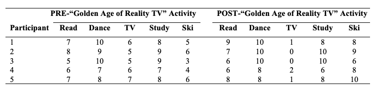
Go to a version of Table 7.2 formatted for accessibility.
Step 1: Enter the Data
- You will need 10 columns to enter the data for each participant. The first five columns will be used to indicate the five pre ratings for the five activities (you can use the data created for Exercise 1 for this but you’d have to rename each variable to indicate they are pre scores). The following five columns will be used to indicate the five post ratings for the same five activities. You should have the following ten variable names Pre Read, Pre Dance, Pre TV, Pre Study, Pre Ski, Post Read, Post Dance, Post TV, Post Study, and Post Ski.Note. In jamovi you can have spaces in your variable names, whereas in other statistics packages sometimes you have to use an underscore instead of a space (e.g., Pre_Read).
- In the Data tab you will need 5 lines in total (one for each participant).
- Be sure to save your data to a suitable place under an appropriate name.
Alternatively you can download the jamovi file (Block 3 Activity 7 Exercise 2 – Two way Within ANOVA.omv; 137kb) with the data entered already for you. After clicking through the link, click on the three dots next to the name and then click Download. From your computer, open this file up (by double clicking on the ‘.omv’ file if you have jamovi installed directly on your computer, or by starting jamovi and then opening the file). Have a careful look at how the variables have been labelled.
Step 2: jamovi for two-way within-participants ANOVA
- Type in or open your relevant data set. Take some time to examine the file, inspecting how the data has been entered and making sure there are no mistakes.
- Select Analyses > ANOVA > Repeated Measures ANOVA… to open the Repeated Measures analysis box.
- In the Repeated Measures Factors box set up our two repeated measures factors with factor and level labels. RM Factor 1 will become PrePost and RM Factor 2 will become Activity.
- Having completed Step 3, the Repeated Measures Cells box should now have labels representing the different combinations of levels across our two repeated measures factors. From the variable list on the left hand side, arrow across the variable that corresponds with each factor level combination according to its label.
- Under Effect Size tick the η2 box.
- Check that under the Model heading the Model Terms box contains both of our RM factors as well as an interaction term. These are the omnibus tests.
- Under the Assumption Checks drop down menu select Sphericity tests, and select Greenhouse-Geisser as well as Huynh-Feldt along with None under Sphericity corrections. We are just including the Huynh-Feldt and none for comparison purposes – with any luck by now you will have learned that it is recommended to always report the results of within-participants ANOVAs with the Greenhouse-Geisser adjustment selected.
- Under Estimated Marginal Means select both RM factors arrow them across to the Marginal Means box one at a time to create Term 1 and Term 2. Click to add a new term then highlight both RM factors at once in the left hand column and arrow them across into one term row for the interaction. Ensure that Marginal means plot and marginal Means table have been selected under Output.
- Finally in order to obtain means and standard deviations, head to the Exploration menu on the Analyses ribbon, click on Descriptives and then select and drag all ten variables across into the right hand Variables box to obtain descriptive statistics for reporting.
Step 3: Examine the output
First let’s check Mauchly’s Test of Sphericity, and epsilon adjustments. Note that we do not get a test for PrePost because there are only 2 levels of this factor. For all two-level factors, there is only one covariance between the levels, so it does not make sense to try to test homogeneity of covariances. The episilon adjustment of 1 for this row means that we multiply the df for the two-level factor by 1, which means it is the same as the raw df.
Figure 7.9
Sphericity Tests in jamovi
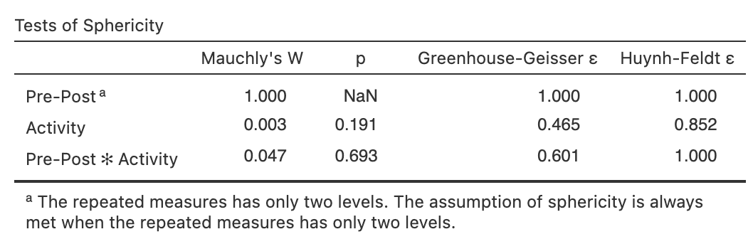
Even though we know the two-level factor is fine, we will need to examine the Mauchly’s test for the tests involving within-participants factors with more than two levels, namely the main effect of the activity factor and the interaction of Activity and PrePost. For these tests, because Mauchly’s test is not robust, we will generally plan to use an epsilon adjustment as a precaution regardless of what Mauchly’s test says – but we still look at the Mauchly’s test as a tradition. 🙂
Next, we review the Tests of ‘Within-Subjects’ Effects table (i.e., the within–participants treatment effects).
Figure 7.10
Within Subjects Effects in jamovi
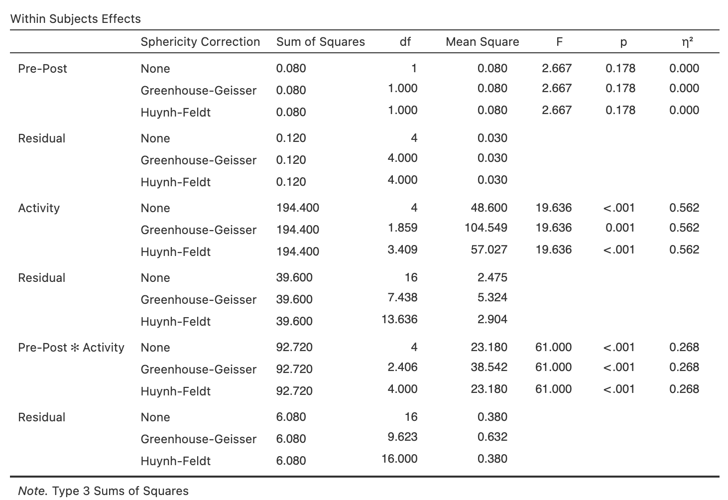
Again, note that because there are only two levels of PrePost, no adjustments are made to the df for this effect.
For the other effects, all the relevant epsilon adjustments have been calculated and tabulated. Furthermore, note that all solutions for these tests of effects provide the same interpretation, which occurs when there is no problem with sphericity in the data.
So, what does this tell us about each of the following treatment effects?
Finally, jamovi then provides the Tests of ‘Between-Subjects’ Effects, i.e., the between participants effect.
Figure 7.11
Between Subjects Effects in jamovi
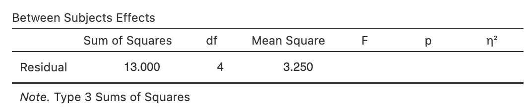
This gives you an estimate of the variance due to?
Click to reveal the answer:
Answer:
Individual differences (a control factor in this design), which we would usually not report because it’s not focal to the research question and also we have a dodgy convenience sample of five people, not a large representative sample which we would seek if we wanted to estimate individual differences instead of just control for them.
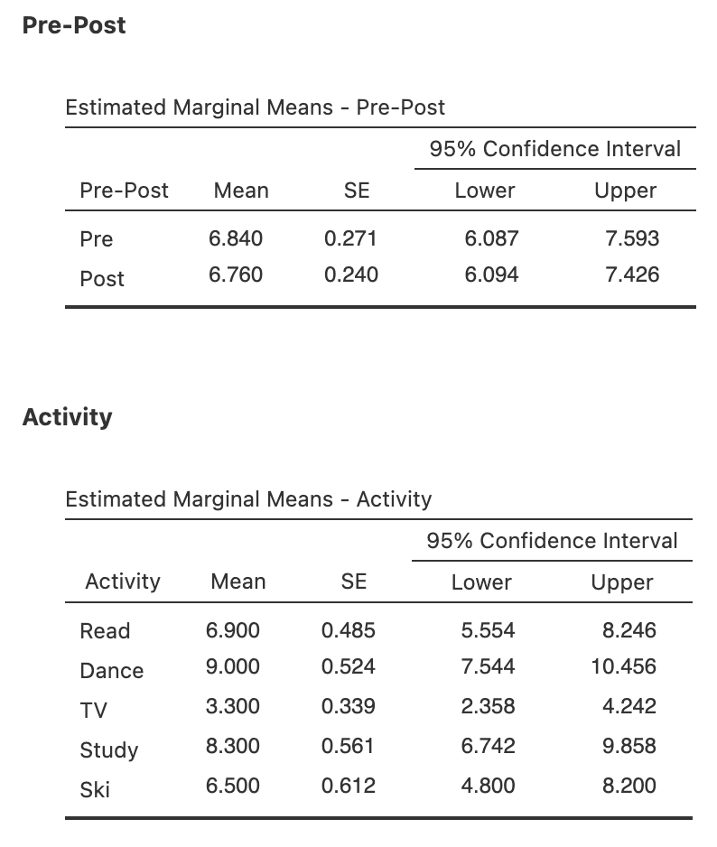
Next, we can look at the marginal means associated with the two within participants factors. The main effect of PrePost was non-significant, so it would not normally be followed up, but we can see the means are nearly the same as each other which is not surprising given the ns result.
The Activity main effect was significant, and the means look very different across the activities. We can see right away the means again are not in the predicted direction: TV viewing seems to attract low satisfaction overall.
Figure 7.12
Marginal Means for the Main Effects of PrePost and Activity in jamovi
Then consider the cell means for the PrePost x Activity interaction (which was significant).
Figure 7.13
Cell Means for the Interaction in jamovi
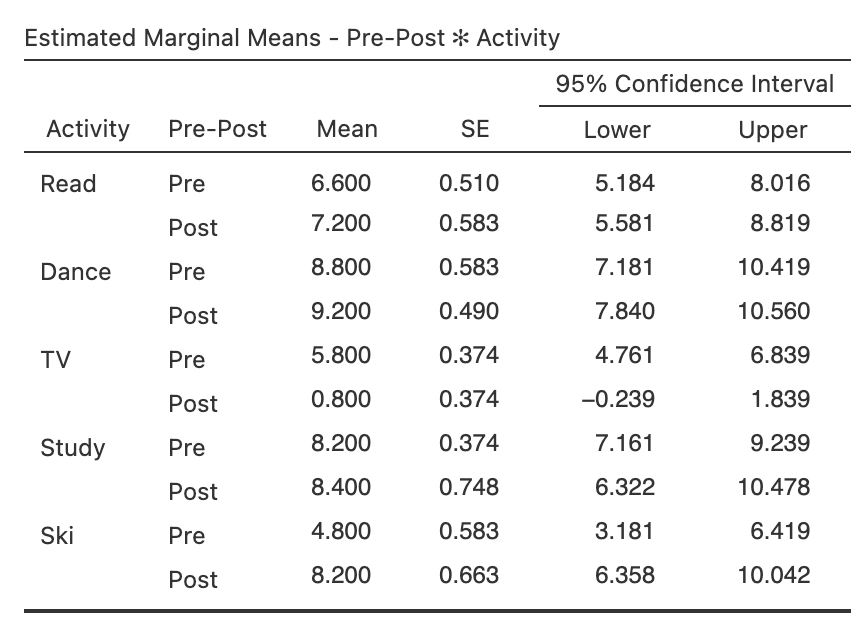
We still have to do the formal follow-up tests, but the pattern in the table is not what was hypothesized: after the introduction of reality television, TV satisfaction is trending down and the other activity ratings are similar or trending up!
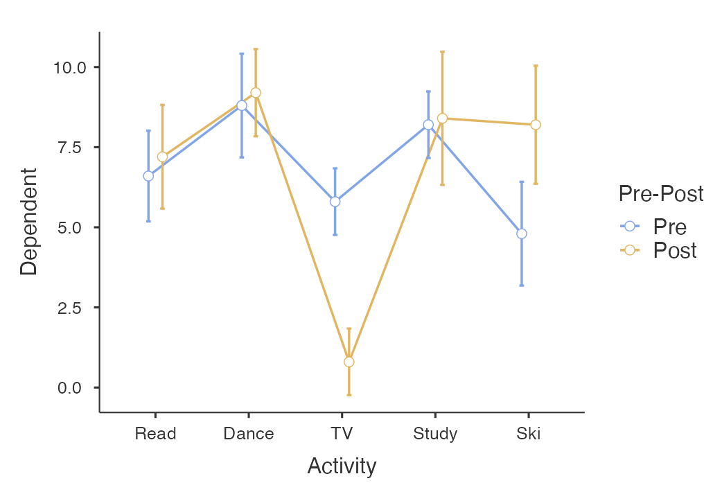
Lastly, jamovi gives you the Plot (i.e., graph) of the PrePost x Activity interaction. Note that the lines are not parallel. This is reflected in the fact that the test of the interaction was significant.
Figure 7.14
Means Plot for Interaction in jamovi
Step 4: Main effect comparisons in a within-participants factorial ANOVA (following up a significant main effect) in jamovi
To follow up the significant main effect of Activity we need main effect comparisons, because we have a factor with > 2 levels. We could compare two theoretically interesting means (e.g., for TV and Study) by selecting only the data that relate to the two trials of interest (i.e., Pre TV, Post TV; and Pre Study, Post Study), running a 2 (PrePost: pre, post) x 2 (Activity: TV, Study) ANOVA and then interpreting only the main effect of Activity (which will average over the two levels of PrePost, and use an error term calculated only from this data).
We have included the relevant tables from the output below:
Figure 7.15
Main Effect of Activity in the Abbreviated Two-Way Within Participants ANOVA in jamovi

Figure 7.16
Marginal Means for Follow-Up Main Effect Comparison from the Activity Main Effect in jamovi
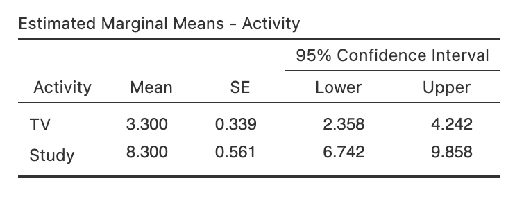
As foreshadowed when we looked at the means, we find that that overall studying is significantly preferred to TV viewing, rather than the reverse.
Step 5: Simple effects in a within-participants factorial ANOVA in jamovi (following up a significant interaction)
Since there is a significant two-way interaction between PrePost and Activity (both within participants factors), we will need to do follow-up simple effect tests. We would need to conduct the simple effects of PrePost for each of the five activities in order to address Hypothesis 2. To do this, we would select Analyses -> T tests -> Paired-Samples T Test… and then highlight each of the five pairs of means (i.e., Pre Read, Post Read etc in pairs) and move them into the Paired Variables box (or you could do this as a one-way ANOVA, with the same p values).
jamovi then presents the 5 paired-samples t-tests.
Figure 7.17
Paired Samples t tests as Simple Effects tests in jamovi
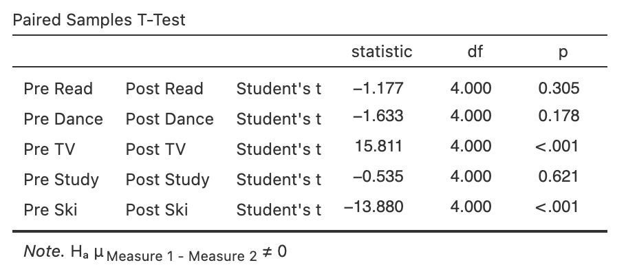
Here we see that after reality TV is introduced, TV viewing satisfaction significantly decreases, and skiing satisfaction increases, with the other three activities showing no significant change (simple effects of PrePost not significant for reading, dance, and study).
Step 6: Complete this summary of the findings, such as might realistically be found in a professionally-written Discussion section of a cutting-edge journal 😉
Note. Effect sizes are not reported in the table above, so you can skip them in your write-up, but normally you would include these as well.
Recommended Extra Readings
Within-participants or repeated-measures ANOVA will be covered in any higher-level statistics textbook; just check the table of contents. For example:
Field, A. (2013). Discovering Statistics Using IBM SPSS Statistics: And Sex and Drugs and Rock “N” Roll, 4th Edition. Sage.
Howell, D.C. (2011). Statistical methods for psychology, 8th edition. Wadsworth.
Test Your Understanding
- In a design involving more than one within-participants variable, a separate error term is needed for each F-ratio. Why is this the case?
- The Greenhouse-Geisser epsilon adjusts the degrees of freedom in an analysis to make the F-test more conservative. Why does adjusting the degrees of freedom make for a more conservative test?
- Sometimes jamovi is unable to calculate the Mauchly’s test result and the associated epsilon values, even though the IV has more than two levels. We think this is for mysterious reasons associated with invariance in at least one of the conditions. If this happens, you would report it in the results, use the unadjusted Fs to report in your write-up, and in the discussion, note that unadjusted results are reported, potentially creating a problem of Type 1 error. This means that there could be a problem of false ______, and replication of the results is desirable to confirm any significant findings.
