
1 Activity 1 – Understanding Factorial Designs and Interactions
Overview
In this introductory section we review the concept of variance and describe how a design can be implemented to address several sources of variance in a dependent variable of interest. We will look at the notion of interacting variables in the context of psychological research, and the role they play in setting up and testing hypotheses.
We then look more closely at what it means for variables to interact. Specifically, we want to look at two levels of analysis – those of main effects and simple effects. The intention of this section is to show how an analysis of simple effects allows us to interpret complex data (in this case interactive data).
Learning Objectives
- Understand the need for complex designs involving several predictors in explaining psychological variables
- Review the concept of variance, and introduce the notion of looking at variance in a dependent measure as potentially reflecting the interplay of multiple variables
- Explain the difference between interactive and additive structures in a set of variables
- Practice graphing and interpreting interactions in complex designs
- Recognise (and be familiar with) the use of main effect and simple effect tests, and their use in interpreting interactions
- Recognise when simple effect tests are appropriate, and how this affects our interpretation of the data
Factorial Designs in Psychological Research
Psychological research is fundamentally about variance. Whatever things we measure, we tend to measure them because they vary – that is, because differences occur. It is these differences that we wish to explain.
Until now, we have made the assumption that differences in a given psychological construct (for example, depression) are related to just one other variable – or factor (for instance the presence or absence of supportive individuals). In other words, we made the simplifying assumption that only one variable was responsible for all the variance in our dependent variable or criterion. Univariate (one-variable) statistics such as Student’s t-test or Pearson’s r do a very good job of testing hypotheses such as these.
But what about the situation where more than one variable can be identified which might influence our measure of interest? There are many situations in which we might wish to test the effects of several independent variables simultaneously on our dependent variable. For these kinds of multi-factor designs, we need techniques which allow us to separate out the components of variance in our dependent variable which might be linked to each independent variable in turn. In this course, we are going to look at a number of techniques to do this.
Interactive Versus Additive Models
Simple, Non-Factorial Designs
Consider a simple t-test. We wish to test the level of people’s statistical knowledge in PSYC3010. We hypothesise that generally, students who have had a high level of previous exposure to maths (e.g., studied complex maths until year 12 or higher) enter the PSYC3010 course with more knowledge of statistics than do students who have had a low level of maths exposure (e.g., studied maths only until year 10). A graph of this effect might look like Figure 1.1 below:
Figure 1.1
The Effect of Previous Maths Exposure Level on Knowledge of Statistics
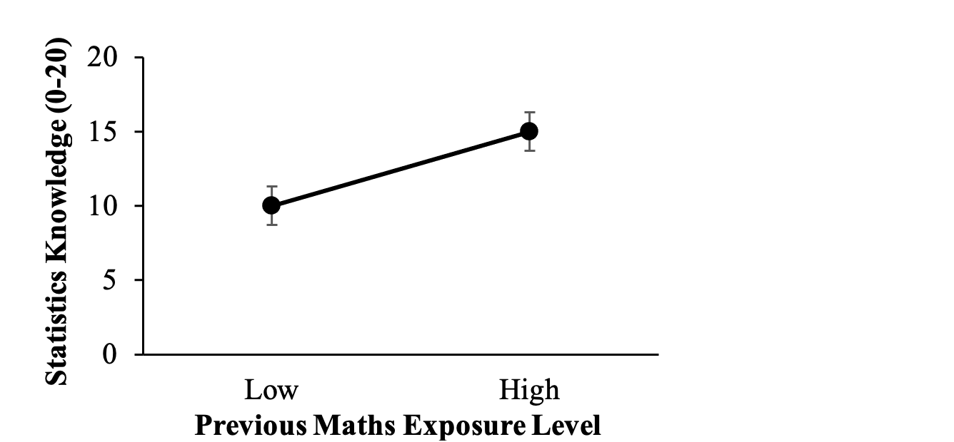
Note. Error bars represent ±1 standard error from the mean.
Factorial Designs: Additive Effects
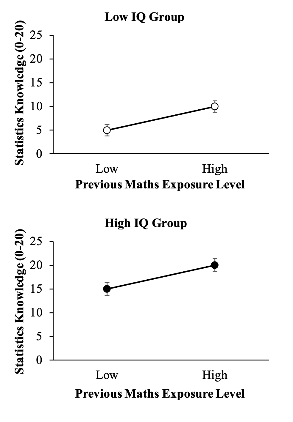
Suppose, however, that we also measured people’s general IQ level and used this as a predictor. We might expect that people who score better on measured tests of intelligence (which gauge much the same qualities as a written test) might also do better on the statistics test. How might these two effects combine? Figure 1.2 below shows the same effect as the last one, but now there are two graphs: one for people with high IQ scores and one for those with low.
Notice that the overall performance of the high IQ group is higher, but that the difference between people who had low and high levels of previous maths exposure is approximately the same magnitude within both IQ groups (i.e., a difference of approximately +5.0).
Figure 1.2
The Effect of Previous Maths Exposure Level on Knowledge of Statistics Plotted Separately for IQ Groups
In Figure 1.3 we have combined these results. We can now see the effects of previous maths level exposure for the low and high IQ groups together in one graph.
This pattern of results, with both groups showing much the same effect, is called an additive effect. This can be seen more clearly if both groups are presented on the same plot, with a separate line for each:
Figure 1.3
The Effect of Previous Maths Exposure Level on Knowledge of Statistics for IQ Groups Plotted Together
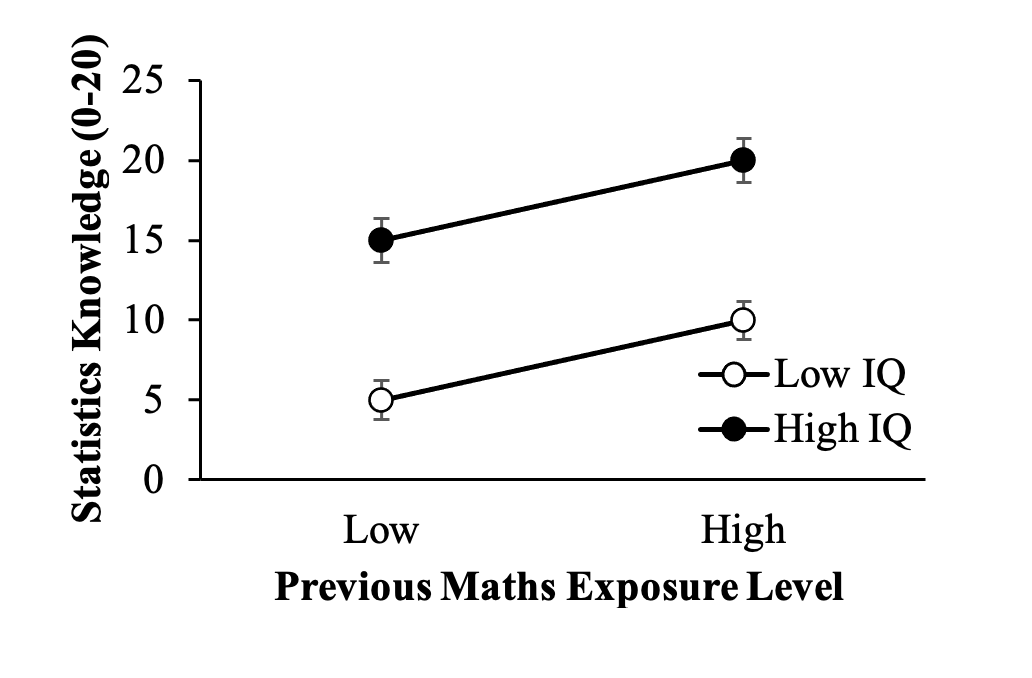
As you can see, the difference in performance between the low versus high previous maths exposure students is of the same magnitude irrespective of IQ level. Although we do note that overall, the higher the IQ, the higher the performance on the knowledge of statistics test.
Factorial Designs: Interactive Effects
By contrast, consider what would be meant by an interactive effect. Imagine we also examined time of assessment, where we tested people once at the beginning of the semester and again at the end. At the beginning we might predict a difference in knowledge of statistics due to previous maths exposure, but these differences will tend to disappear over time as all students become more familiar with the work involved in PSYC3010. Such a pattern might look like Figure 1.4:
Figure 1.4
The Effect of Previous Maths Exposure Level on Knowledge of Statistics by Time of Assessment
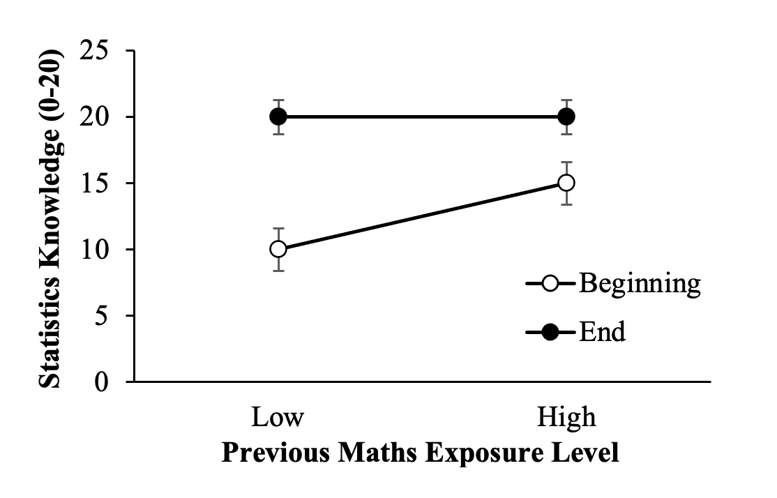
Notice that the lines are no longer parallel? This is a visual sign that the effects are interactive, not additive. In other words, the knowledge difference between students with low and high levels of previous maths exposure in this instance depends on the time of assessment (i.e., whether they were measured on statistics knowledge at the beginning or end of their PSYC3010 semester).
We will be talking a lot about the distinction between additive and interactive effects, and how to handle them.
The Meaning of an Interaction
As you can see, an interaction between two variables is present whenever the effect of one of the variables differs at different levels of the other variable. In other words, an interaction is present whenever you can describe an effect with the words “it depends”. For example, the effect of previous maths exposure on statistics knowledge depends on the time of assessment.
Take another example: your doctor hands you a prescription and tells you to be careful because the drug interacts with alcohol. This means that the effect of the drug will depend on whether you consume alcohol or not. So, when you do not consume alcohol, taking the prescription will help you. However, when you do consume alcohol, taking the prescription will not help – or perhaps even harm – you.
Interactions are of primary importance in psychological statistics, and so the next section will consider various kinds of interactions and the patterns of data they can create.
Levels of Analysis in Complex Designs
To understand more thoroughly why we need factorial designs, consider the following statement: any hypothesis you can propose is a kind of generalisation. To say that students who completed year 12 maths (i.e., have “high levels” of previous maths exposure) are always better at statistics is a sweeping generalisation. In reality, it shouldn’t need to be pointed out that it depends on the particular student involved. If we broke it down and looked at students with high or low levels of previous maths exposure who had completed a unit of PSYC3010, versus those who had not (as in Activity 1), we might find that a different picture holds for each previous maths exposure group.
These two different levels of analysis, therefore, give a different picture of the data. On the one hand, looking at students overall, you can tell one kind of story. Yet looking at each group separately, you can tell another.
Basically, a Main Effect is the level of analysis where we examine only one factor at a time. To look at the main effect of previous maths exposure, we look at all the individuals together, and ask “overall, do the students with higher levels of previous maths exposure perform better than students with low levels of previous maths exposure?”
The Simple Effect of a variable is the effect of that variable at each level of the other variable. If we ask “what is the effect of previous maths exposure on students at the beginning of the semester, who have just enrolled in PSYC3010?” or “for those at the end of semester who have just completed PSYC3010, what is the effect of previous maths exposure?”, each of these questions would be assessed with a simple effect (i.e., the simple effect of previous maths exposure at the beginning time of assessment level, and the simple effect of previous maths exposure at the end time of assessment level, respectively).
Main Effects
Consider the imaginary data for our hypothetical experiment shown in Table 1.1 below. Imagine that each cell contains the average (i.e., mean) score for a given group at a given time. Thus, the low maths exposure students at the beginning of the semester had a mean score of 10.
Table 1.1
The Effect of Previous Maths Exposure Level and Time of Assessment on Knowledge of Statistics
|
Level of Previous |
Time of Assessment |
|
|
Maths Exposure |
Beginning |
End |
|
Low |
10.0 |
20.0 |
|
High |
15.0 |
20.0 |
Go to a version of Table 1.1 formatted for accessibility.
We could look at the main effect of previous maths exposure by ignoring the time of assessment variable altogether. All we would have to do is average (or collapse) across the two time points, like you can see in Table 1.2.
Table 1.2
The Effect of Previous Maths Exposure Level and Time of Assessment on Knowledge of Statistics with the Main Effect of Previous Maths Exposure Level
|
Level of Previous |
Time of Assessment |
M |
|
|
Maths Exposure |
Beginning |
End |
|
|
Low |
10.0 |
20.0 |
15.0 |
|
High |
15.0 |
20.0 |
17.5 |
Go to a version of Table 1.2 formatted for accessibility.
Each of these new values (i.e., 15.0 and 17.5) is what we call marginal means.
The marginal means are what we compare in main effects tests. We could use these marginal means of previous maths exposure to make a new table, like Table 1.3 below:
Table 1.3
The Main Effect of Previous Maths Exposure Level on Knowledge of Statistics
|
Level of Previous |
M |
|
Maths Exposure |
|
|
Low |
15.0 |
|
High |
17.5 |
Go to a version of Table 1.3 formatted for accessibility.
As you can see, looking at the whole/overall group, students who had high levels of previous maths exposure did indeed do a little better than students with low levels of previous maths exposure on the statistics knowledge test.
Now let’s consider how we would look at the main effect of the time of assessment variable, our second IV. Again, we would simply average (or collapse) across the other factor, in this instance, previous maths exposure. This gives us Table 1.4 below.
Table 1.4
The Effect of Previous Maths Exposure Level and Time of Assessment on Knowledge of Statistics with the Main Effect of Time of Assessment
|
Level of Previous |
Time of Assessment |
|
|
Maths Exposure |
Beginning |
End |
|
Low |
10.0 |
20.0 |
|
High |
15.0 |
20.0 |
|
M |
12.5 |
20.0 |
Go to a version of Table 1.4 formatted for accessibility.
Which we could present as Table 1.5 showing the marginal means for time of assessment:
Table 1.5
The Main Effect of Time of Assessment on Knowledge of Statistics
|
|
Time of Assessment |
|
|
|
Beginning |
End |
|
M |
12.5 |
20.0 |
Go to a version of Table 1.5 formatted for accessibility.
This second main effect tells us that overall, people performed a lot better at the end of the semester than at the beginning. Recall that we have averaged across previous maths experience, so that at this level of analysis, we are talking about everybody’s performance.
Basically, then, you can see that main effect tests show us the effects of each factor ignoring the influence of the other factor (by averaging over that other factor). By contrast, simple effect tests allow us to examine the effects of a factor at each level of the other factor. This level of analysis (simple effects) is more useful when looking at and trying to understand interactions.
Simple Effects
Let us imagine that in the example above we wanted to look at the effect of previous maths exposure separately for those beginning the semester, and for those who have completed the PSYC3010 course (i.e., at the semester’s end). For this level of analysis, we need to look at the cell means rather than the marginal means. Thus, to look at the effect of previous maths exposure just for those who are beginning the semester, we would compare the means only for that group. Hence, our original table as reproduced here as Table 1.6.
Table 1.6
The Effect of Previous Maths Exposure Level and Time of Assessment on Knowledge of Statistics
|
Level of Previous |
Time of Assessment |
|
|
Maths Exposure |
Beginning |
End |
|
Low |
10.0 |
20.0 |
|
High |
15.0 |
20.0 |
Go to a version of Table 1.6 formatted for accessibility.
This becomes Table 1.7.
Table 1.7
The Simple Effect of Previous Maths Exposure Level when Tested at the Beginning of Semester
|
Level of Previous |
Time of Assessment |
|
Maths Exposure |
Beginning |
|
Low |
10.0 |
|
High |
15.0 |
Go to a version of Table 1.7 formatted for accessibility.
The difference between these two cell means gives us our simple effect of previous maths exposure for those at the beginning of the semester (i.e., the effect of previous maths exposure at one level of time of assessment – as opposed to averaged over all the time of assessment levels). The simple effect of previous maths exposure for those at the end of the semester would look like Table 1.8.
Table 1.8
The Simple Effect of Previous Maths Exposure Level when Tested at the End of Semester
|
Level of Previous |
Time of Assessment |
|
Maths Exposure |
End |
|
Low |
20.0 |
|
High |
20.0 |
Go to a version of Table 1.8 formatted for accessibility.
When a variable’s simple effects are eliminated or change direction or strength depending on the level of the other variable, that variable’s effects are qualified by the other variable. In this example, we would say that the main effect of previous maths exposure is qualified by time of assessment: students with high levels of previous maths exposure performed better on measured statistics knowledge than those with low levels of exposure at the beginning of the semester. But there was no difference in performance between those with low and high levels of previous maths exposure at the end of semester. That is, the simple effect of previous maths exposure seen at the beginning of semester was eliminated or nullified at the end of semester. Whenever the simple effect of a variable is not the same at all levels of the other variable, we know we have an interaction present (this is what causes the non-parallel lines on the graph).
Deciding on the Level of Analysis
Deciding which level of analysis is appropriate can be complex. In general, we start our analysis of two independent variables by conducting the main effect tests and the interaction test. These are called the “omnibus” tests (Latin for “for all”). If the interaction test is not significant, however, you should not perform tests of the simple effects.
Recall that variables can be either additive or interactive. If the variables do not interact, this means that the effect of one variable is consistent at all levels of the other variable, and vice versa. Thus, it is not necessary to look at each simple effect individually: the main effect describes the data well. Whenever there is an interaction, however, we follow up the significant interaction by examining the simple effects. We need to examine the simple effects to explore just what that interaction means – how one variable’s effect changes depending on the level of the other variable.
Exercise 1: 2 x 2 Between Groups (Independent Groups) Factorial Design
The Effects of Source Expertise and Induced Mood on Agreement
An experimenter wishes to explore the effects of source expertise (non-expert or expert) and induced mood (negative or positive) on agreement with a persuasive message (with agreement measured on a 9-point scale). All participants heard a message about pollution and were persuaded to make changes in their everyday life to minimise their own impact on the environment (e.g., reduce, reuse, recycle and replace). This message was either delivered by a non-expert (a scientist studying child development) or an expert (a scientist studying the effects of global warming). Participants heard the message while either in a negative or positive mood. To induce a negative mood, prior to participants hearing the message, the researcher asked them to take five minutes to think about the least pleasant thing that happened to them in the last week. To induce a positive mood, the researcher asked participants to think about the most pleasant thing that happened to them in the last week. The researcher used a 2 (source: non-expert, expert) x 2 (mood: negative, positive) between groups factorial design. The 40 participants were randomly allocated to one of the four experimental conditions, such that there were 10 participants in each.
The following tables present a range of hypothetical outcomes for the above Source x Mood experiment. In practice, the significance of the main effects and interaction is assessed by means of an F ratio. You haven’t learned how to calculate F tests in factorial ANOVA yet, so for this exercise we will simply “eyeball” the data. That is, we will look at the graph and examine the marginal and cell means to give us an indication of what effects might be significant.
For this exercise, we will use the following criteria:
- MAIN EFFECT OF SOURCE = a difference between the column marginal means.
- MAIN EFFECT OF MOOD = a difference between the row marginal means.
- INTERACTION = if the lines on the graph are not parallel. That is, if the size of the difference in cell means for non-experts versus experts is different when participants were in a negative mood compared to a positive mood, then there is an interaction. Similarly, if the size of the difference in cell means for negative versus positive mood is different when participants heard a non-expert compared to when they heard an expert, then there is an interaction.
Enter your answers for the following questions. You can export your responses to a Word document:
Exercise 2: 4 x 2 Between Groups Factorial Design
The Effects of Caffeine Dose and Sex on Spelling Test Performance
A researcher is interested in the effect of caffeine dosage and sex on performance on a spelling test. They recruit male and female participants and randomly assign them to a particular caffeine dosage (zero, small, moderate, large), before measuring their performance on a spelling test (scored out of 20).
Enter your answers for the following questions:
Line Graphs versus Bar Graphs
The data we are using could be displayed using line graphs or bar graphs. For example, the exact same data could be presented in the following two ways*:
Figure 1.5
The Effect of Caffeine Dosage on Spelling Performance by Sex
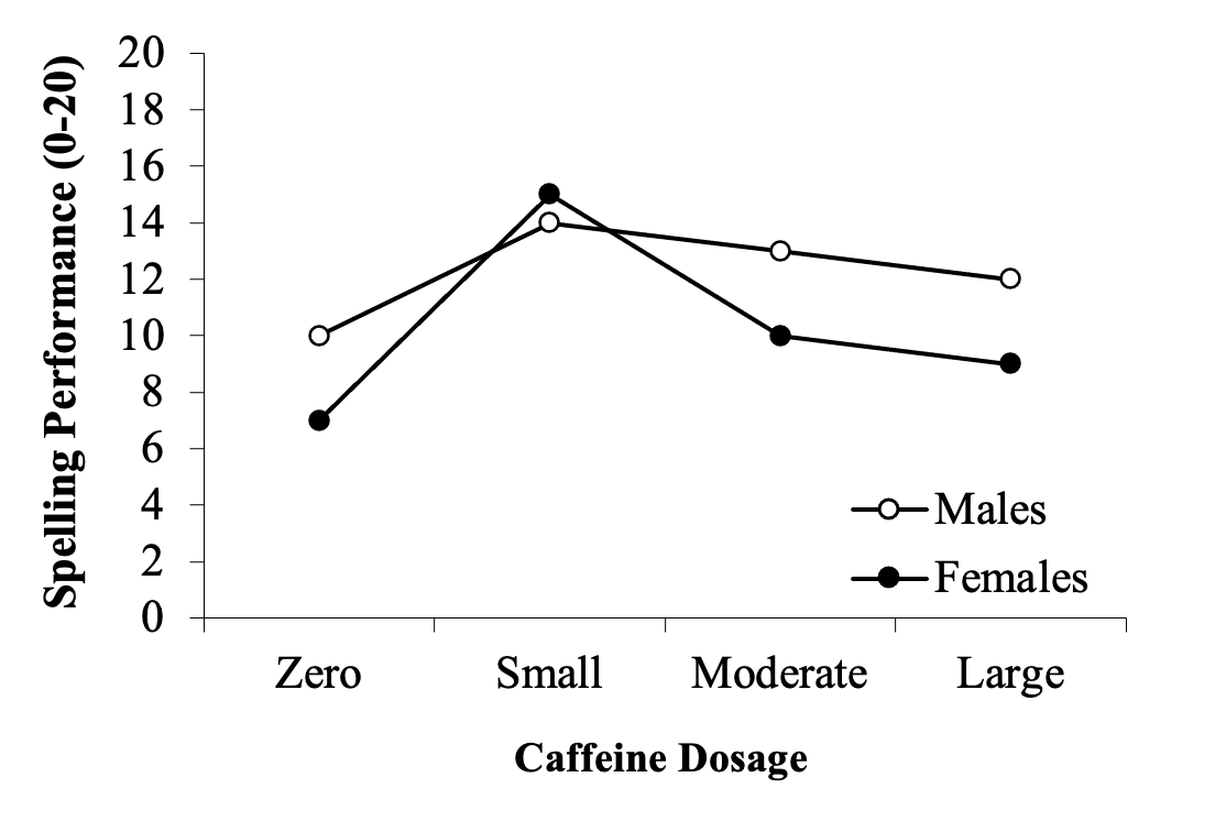
Figure 1.6
The Effect of Caffeine Dosage on Spelling Performance by Sex
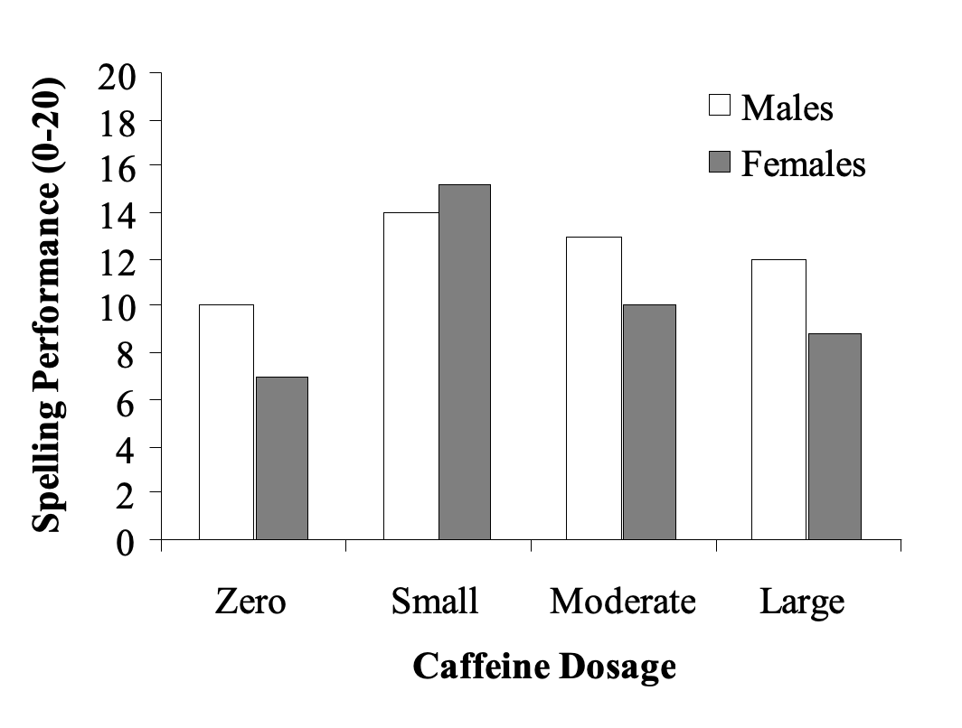
* Note that there are no error bars on either of these two graphs, as the necessary data to calculate these was not given (i.e., we have the means for each group only, not the individual scores. Therefore, we cannot calculate either the standard deviations or standard errors associated with these means). APA 7th format requires that error bars be presented on graphs.
We prefer using line graphs in this course because we find it makes detecting and understanding interactions easier and clearer, respectively.
But the rules technically state that line graphs should be used for continuous IVs, whereas categorical IVs should be represented on bar graphs. In this course, you can use either for your assignments. We will continue to use line graphs in this booklet because of their illustrative quality.
Recommended Extra Readings
It’s a very personal choice…
Heiman, G. W. (2011). Basic statistics for the behavioral sciences (Chapter 14, pp. 318-350). Wadsworth, Cengage Learning.
Schweigert, W. A. (1994). Research methods and statistics for psychology (Chapter 9, pp. 286-287). Brookes/ Cole.
Tilley, A. (1996). An introduction to psychological research methods and statistics (Chapter 14, pp. 377-392). Pineapple Press.
Test Your Understanding
- Consider the psychological construct of extroversion. Think of at least two (2) variables that might be used to predict extroversion. On your own reasoning, do you think that their effects would be additive, or would they interact? Why?
- A researcher was interested in looking at the effects of various kinds of antibiotics in treating acne. They administered three kinds of antibiotics and discovered that for some people none were effective. For others, each of the antibiotics had some effect, but drug C was clearly superior to drugs A and B. Questioning their participants, the researcher discovered that the difference between people who had responded to the drugs and those who had not, was that those who failed to respond had consumed alcohol at some stage during the testing (which took several weeks). What kind of design should the researcher use to test the efficacy of the drugs? Would they expect to find an additive or interactive effect?
- Consider the following example: a sport psychologist hypothesised that both body type (ectomorph, endomorph, mesomorph) and motivation level would play a role in people’s high-jump performance. How would they set up an experiment to test this? Graph the expected results and indicate whether the variables would be additive or interactive.
- Explain the difference between a main effect and a simple effect. Use an example to illustrate your answer.
- A researcher hypothesised that the relationship between weight loss and the amount of exercise a person does depends on the kind(s) of exercise undertaken. Specifically, they hypothesised that those who undertake primarily aerobic exercise will lose weight as a function of the amount of exercise they perform; whereas those who undertake primarily muscle intensive exercise (such as weight training) will gain weight as a function of the amount of exercise they perform. Design an experiment which tests these hypotheses. What omnibus tests would be needed to address these questions? Would simple effects or comparisons be needed? If so, outline what set of follow-up tests you would perform.
- Consider the following relationship:
Figure 1.7
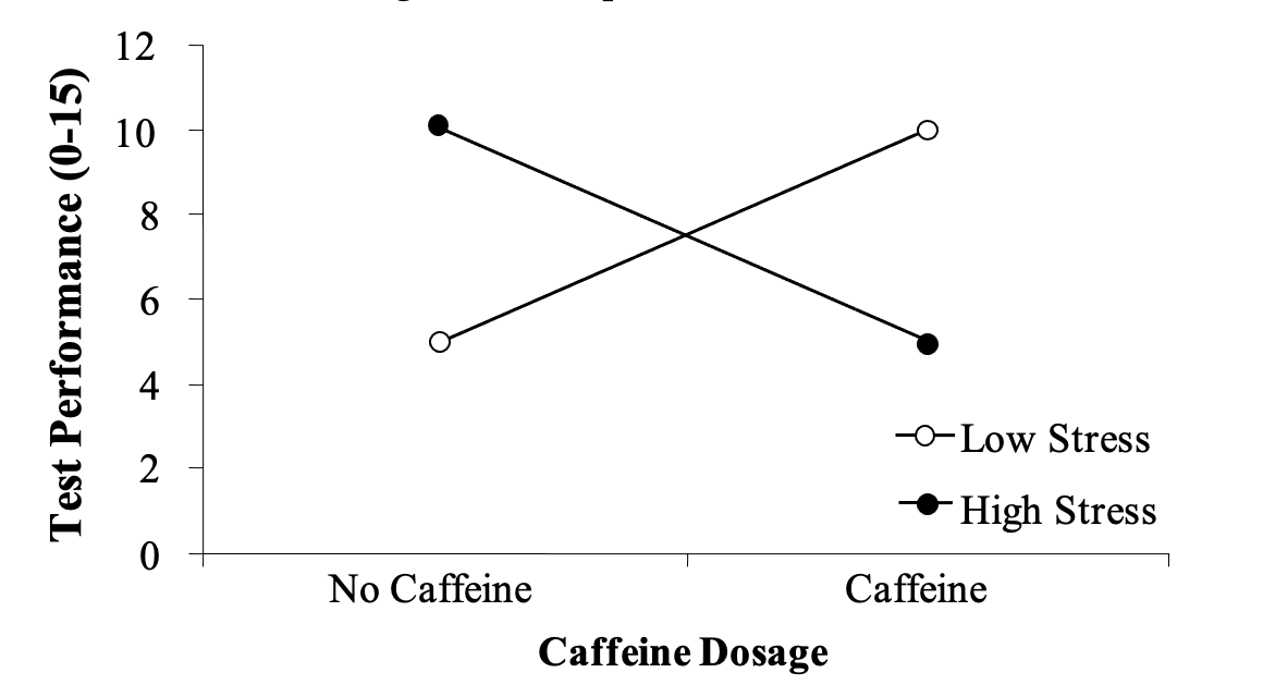
The two IVs in this experiment are caffeine dosage (no caffeine, caffeine) and stress level (low, high). What kind of study design is this? Based on the figure, which omnibus effects do you think would be significant? Which simple effects would be significant? Explain your answer.
