
2 Activity 2 – Between Groups (a.k.a. Independent Groups) Factorial ANOVA: Omnibus Tests in jamovi
Last reviewed 19 December 2024. Current as at jamovi version 2.6.19.
Overview
In this section, we review the meaning of the F-ratio used in ANOVA. We then introduce the jamovi statistical package and examine the procedures for running a two-way between groups (independent groups) factorial ANOVA, focusing on the omnibus tests.
Learning Objectives
- To understand how variance is partitioned in two-way between groups factorial ANOVA
- To introduce the jamovi statistical package
- To practice entering data in jamovi, and to conduct the omnibus tests in a two-way between groups factorial ANOVA
- To interpret the jamovi output from a two-way between groups factorial ANOVA
- To write up results of the omnibus tests from a two-way between groups factorial ANOVA
A Review of the Logic of ANOVA: The One-Way Case
In the examples we covered in the previous section, we looked at how you could design a factorial experiment by allocating people to different groups, each of which represented a different combination of levels of our variables of interest. To analyse these kinds of between groups designs, we are going to employ a between groups factorial ANOVA, which is basically a straight-forward extension of the one-way between groups ANOVA that you have already studied in previous statistics courses at UQ.
Recall that the basic design of the ANOVA involves partitioning the observed variance in the DV into two “sources” – that which is attributable to the variable of interest (treatment), and the rest, which we have simply called “error”. So, the basic design is illustrated in Figure 2.1 below:
Figure 2.1
Partitioning of Variance in ANOVA
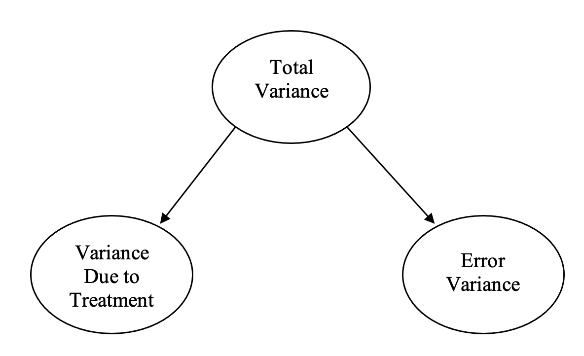
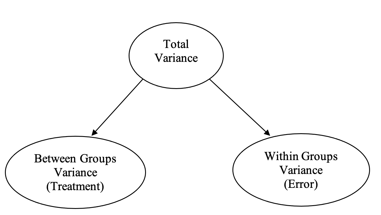
The F-ratio is the ratio of explained variance (i.e., treatment variance) to error variance, and is evaluated for significance. In terms of actual numbers, the variation due to treatment is estimated by the difference between the scores for each group, whereas the variation due to error is estimated by the differences in people’s scores within each group. So for a between groups ANOVA we have something like Figure 2.2:
Figure 2.2
Partitioning of Variance in a One-Way Between Groups ANOVA
Extension to the Two-Way Case
When we have two independent variables, we are able to account for more of the variance in our DV. As a result, the “error” component is smaller. So, in effect, we are identifying more actual sources of the variance in the DV.
Consequently, in a two-way between groups ANOVA, we now partition the total variance into four sources as shown in Figure 2.3 below:
Figure 2.3
Partitioning of Variance in a Two-Way Between Groups ANOVA
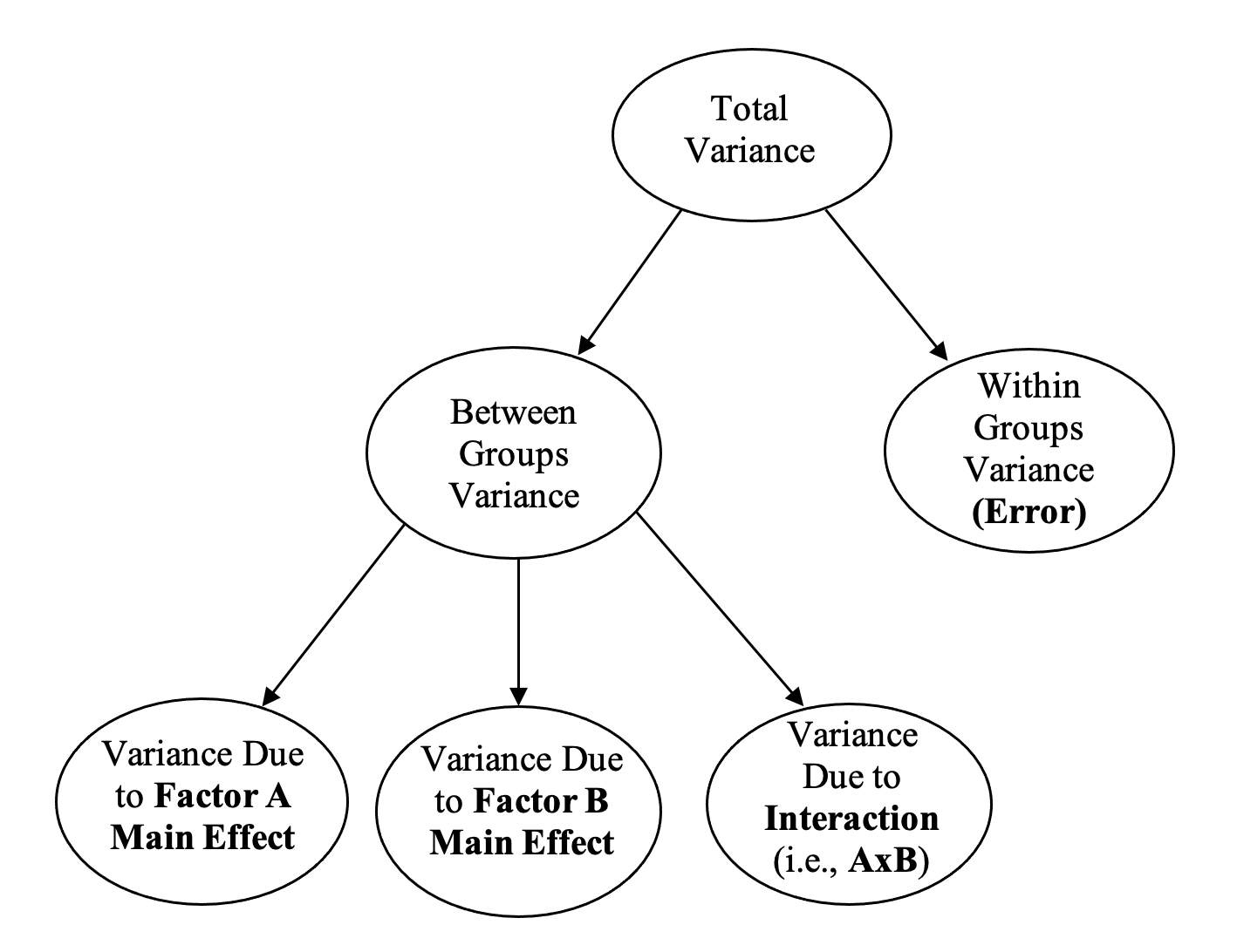
The between groups variance (i.e., treatment variance) is now partitioned into three (3) separate sources:
- the variance between groups on factor A,
- the variance between groups on factor B, and
- the remaining variance between the groups, which represents our interaction between factors A and B (which we write as “AxB”).
The within groups variance (i.e., the differences between people’s scores within the same group) still forms our error term.
Activity 2 Exercise 3: 4 x 2 Between Groups Factorial Design
Sex, Drugs, and Rats…
A psychologist is interested in the effect of four different dosage levels of a steroidal drug and sex on physical performance (maze running) of laboratory rats. They take 20 male and 20 female rats, and randomly assign them to one of four conditions that vary in the dosage of the drug (zero, small, moderate, large). They then measure the rats’ physical performance on a scale from 1 to 15 (with higher scores indicating better performance). The researcher reasons that different drug dosages may affect maze running ability; that male and female rats may differ in performance; and that certain drug dosages may affect maze running performance more for one sex than for the other. Based on what they know about the effect of this drug, the researcher makes the following specific hypotheses:
- Overall, male rats will outperform female rats on maze running.
- Overall, rats will perform better when they receive any amount of the drug than when they do not receive the drug.
- However, a small dose will tend to lead to the best performance compared to a large dose.
- The effect of drug dosage will differ for males compared to females. While both sexes will exhibit increased performance when they receive any amount of the drug than when they do not, the particular benefits of the small drug dosage (compared to the large dose) will be more noticeable in female rats than in male rats.
1. Before performing any analyses, decide which omnibus statistical results will address each hypothesis.
2. Examine the following table containing our data. We have added the marginal and cell totals and means to help you identify potential main/ simple effects.
Table 2.1
The Effect of Steroidal Dosage and Sex on Maze Running Performance in Rats
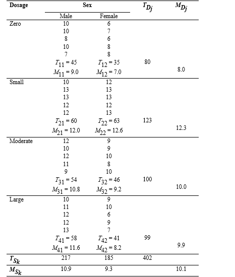
Go to a version of Table 2.1 formatted for accessibility.
3. Using the axes below, plot the cell means and think about what results to expect in terms of the omnibus tests (i.e., are we expecting a significant main effect of sex, main effect of drug dosage, and/ or Dosage x Sex interaction?).
We will now introduce the jamovi statistical package in order to learn how it can help us analyse large data sets quickly and easily.
Accessing jamovi
If you are on campus you can access jamovi in HABS faculty computer labs.
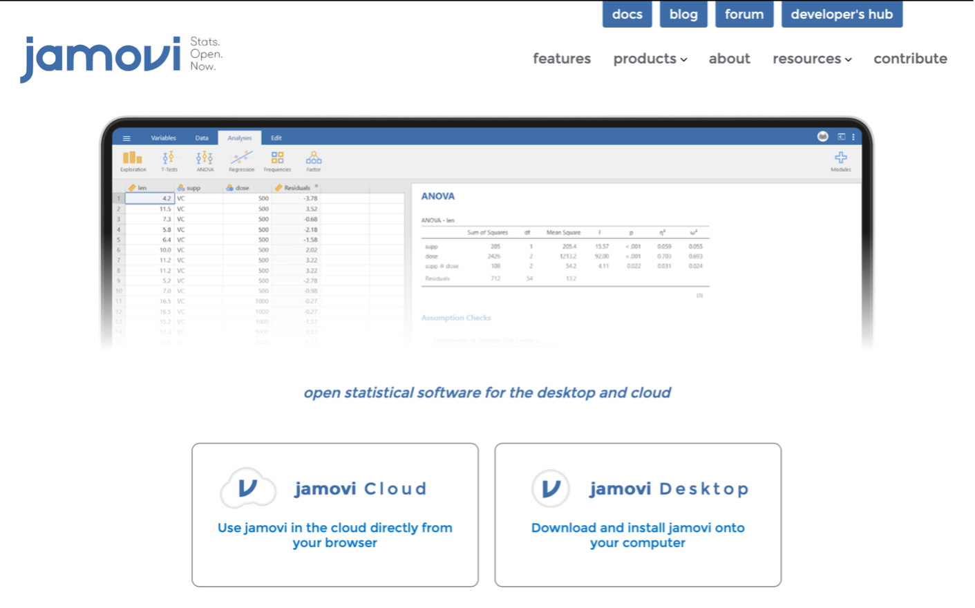
If you are wanting to conduct your analyses on your own device you will need to either download the jamovi desktop program or access the jamovi cloud browser version. The desktop version is available for Windows, macOS, Linux, and ChromeOS. If your device has a different operating system, or you do not wish to download and install the program, you can use the jamovi cloud browser version. The cloud version is less desirable though because there is a cap on the number of users for the free version and if too many other people are online, sometimes jamovi will not work. This limitation does not affect you if you have the desktop version, so we recommend the desktop version as the first choice.
Head to the jamovi website to download or access the jamovi statistical package.
Figure 2.4
The jamovi website
The jamovi Statistical Package
Once you have the jamovi statistical package installed on your computer (or the browser-based version up and running you can open the data file we’ll be using in this activity and the next.
Download the Factorial BG ANOVA starting data file (omv, 2 KB).
1. Data Entry and Editing
The first essential components of the jamovi statistical package are the “Variables” and “Data” tabs which together allow you to enter data and specify the name and nature of your variables.
1a. The Variables View
Before typing in our actual data values, we first need to set up our variables of interest. We do this in the Variables tab, which is the first tab on the left. In the Variables tab (see below), we name and label our IVs and DVs, as well as assign value labels to the levels of all our discrete variables (this does not need to be done for continuous variables). We will do all this in just a few moments in Exercise 4.
Figure 2.5
The Variables Tab in jamovi
1b. The Data View
To type data into the jamovi for analyses, we enter the numbers into the Data tab. Note that as we type in our data using our numeric values, jamovi will display the value label that corresponds with that numeric value.
Figure 2.6
The Data Tab in jamovi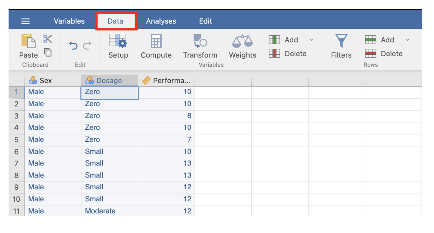
2. Selecting Analyses to Run
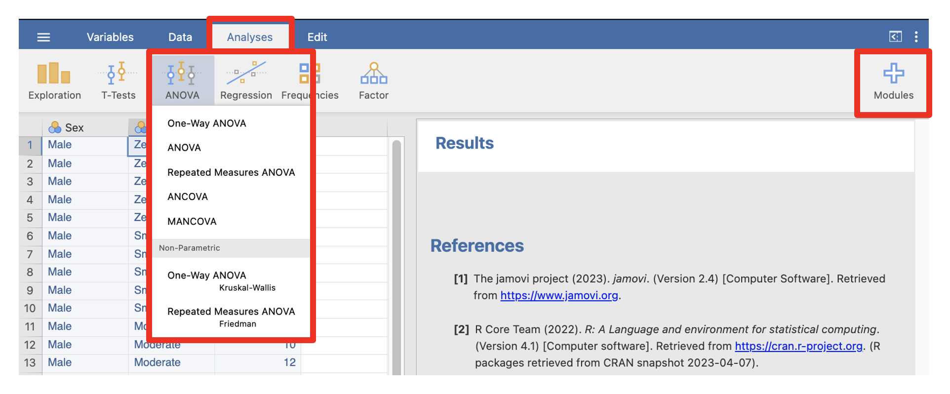
Once we have set up our variables and entered the data, we need to actually conduct the analyses. jamovi loads with a base selection of menus in the analyses tab as is highlighted in red below. However, there are many other modules that can be added via “+ Modules” menu that can be seen on the far right hand side of the menu ribbon. Each analysis grouping has a number of analyses that can be selected from a drop-down menu as is shown below:
Figure 2.7
The Analyses Tab in jamovi
3. The Results Window
The output (i.e., results) appears in the right hand side of the jamovi program window and dynamically updates as you select each analysis option. When you click in any part of your results output, the menus and chosen options that created it will appear on the left hand side of the program window.
Figure 2.8
The Results Window in jamovi
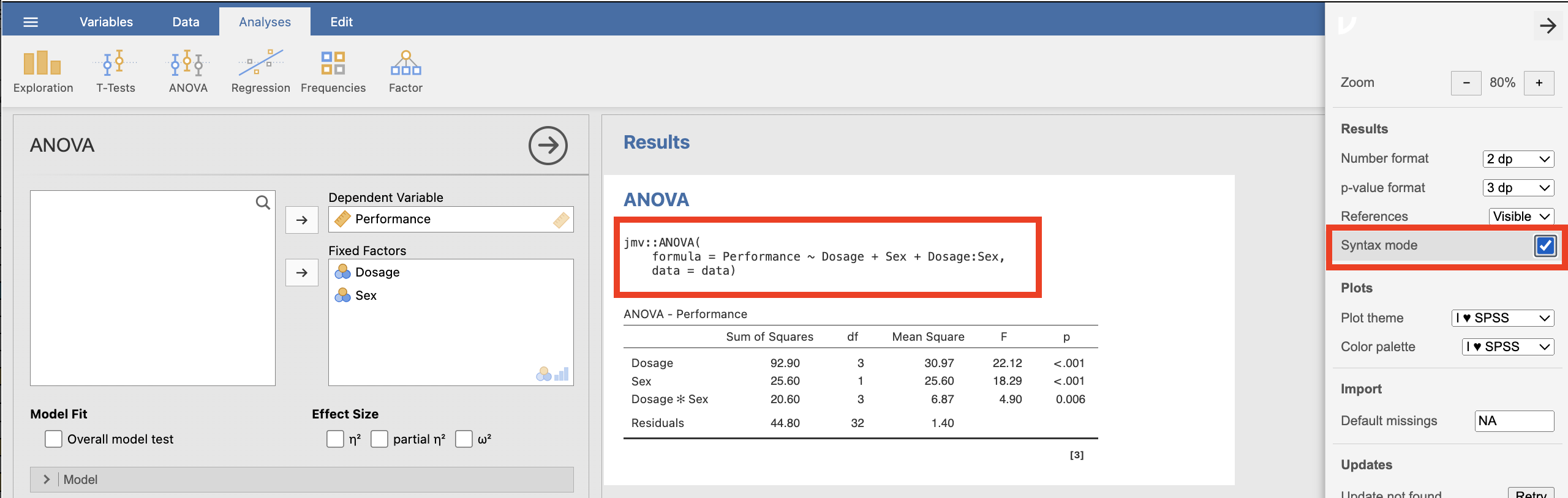
4. The Syntax Mode
The jamovi statistical package can be a stepping stone to gaining familiarity with another widely used and highly versatile open-source statistical package known as R. In R we use coding or “syntax” to specify what we want to do. You can activate the “Syntax Mode” in jamovi which will then provide you with the R code that underlies the analyses you have conducted.
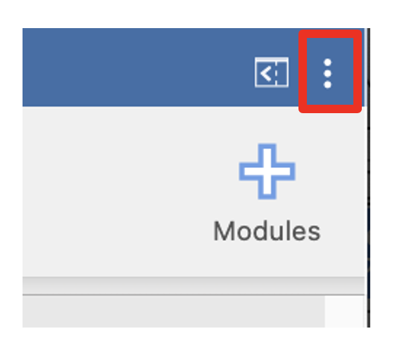
There is a settings menu that can be found by clicking on the three vertical dots on the far right side of the menu ribbon.
Figure 2.9
Accessing the Settings Menu in jamovi
When you click this, various settings will appear and you will see there is a check box you can tick to turn on syntax mode. With syntax mode activated, as shown in the screenshot below, you will be provided with the R code for the analysis above the results.
Figure 2.10
Activating Syntax Mode in jamovi
Activity 2 Exercise 4: 4 x 2 Between Groups ANOVA in jamovi
We will use the rat Drug Dosage x Sex experiment to conduct a 4 x 2 between groups factorial ANOVA in jamovi. Here is the raw data that you will need to type into jamovi for this exercise:
Table 2.2
The Effect of Steroidal Dosage and Sex on Maze Running Performance in Rats
|
|
Sex |
|
|
Dosage |
Male |
Female |
|
Zero |
10 10 8 10 7 |
6 7 6 8 8 |
|
Small |
10 13 13 12 12 |
12 13 13 12 13 |
|
Moderate |
12 10 12 11 9 |
9 9 10 8 10 |
|
Large |
10 11 12 12 13 |
9 10 6 9 7 |
Go to a version of Table 2.2 formatted for accessibility.
Step 1: Enter the Data
A jamovi data spreadsheet contains one line of data for each participant (in this case, rat). You’ll need three columns to enter the data – the first column will identify what level the participant is in for the sex factor (i.e., male or female), the second column will identify the participant’s level on the drug dosage factor (i.e., zero, small, moderate or large), and the third column will record the participant’s maze running performance score.
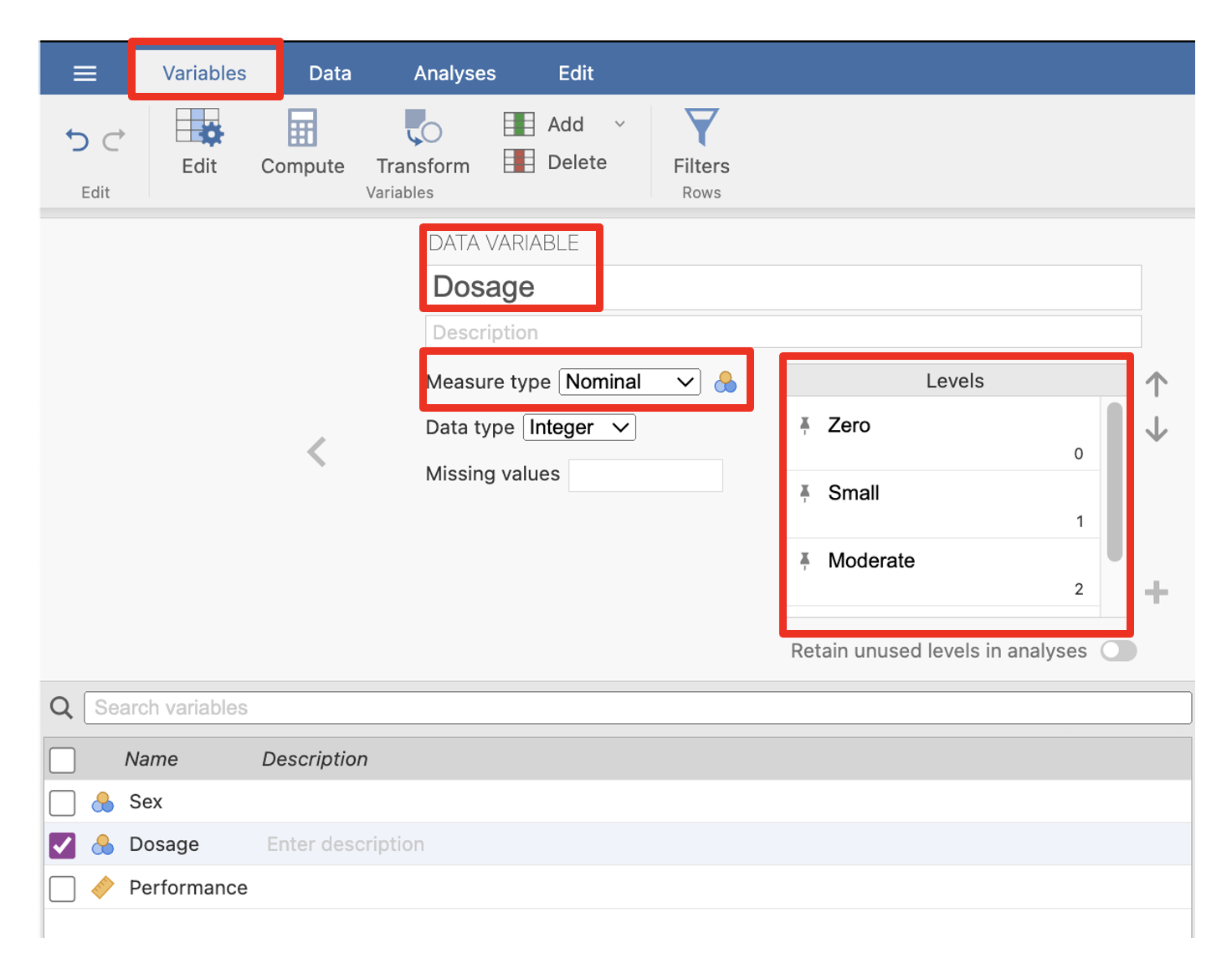
- To specify the variables, click on the Variables tab. In the Variables tab each row represents a variable. In the first row in the Name column, type in the name of the variable with the fewest levels – Sex. Using the variable with the fewest levels first makes data entry easier (which you will see in a moment).
- If you want to give your variable a longer name than what is allowed in the Name column, you also have the option of typing in a longer name in the Description column. We don’t really need this because we have enough space to type a descriptive name in the Name column.
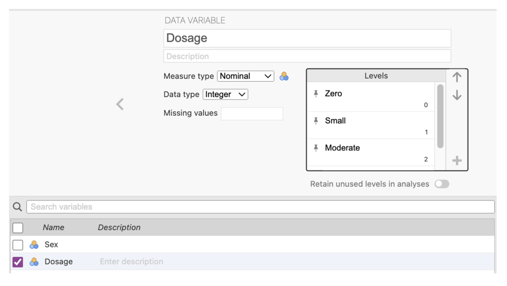
- Click on Variables > Edit in the menu ribbon to reveal where you can add details such as the level of measurement of the variable as well as values and associated labels.
Select Nominal in the Measure type list.
Next to the “Levels” box type click on the + and in the pop-up box, type in the first value of 1. Then click on the + again and type in the second value of 2.
Click in the row with the value of 1 and type in the value label male, then click in the value of 2 and type in the value label of female.
The end result should like the screenshot below.
Figure 2.11
Sex Variable Specification in jamovi
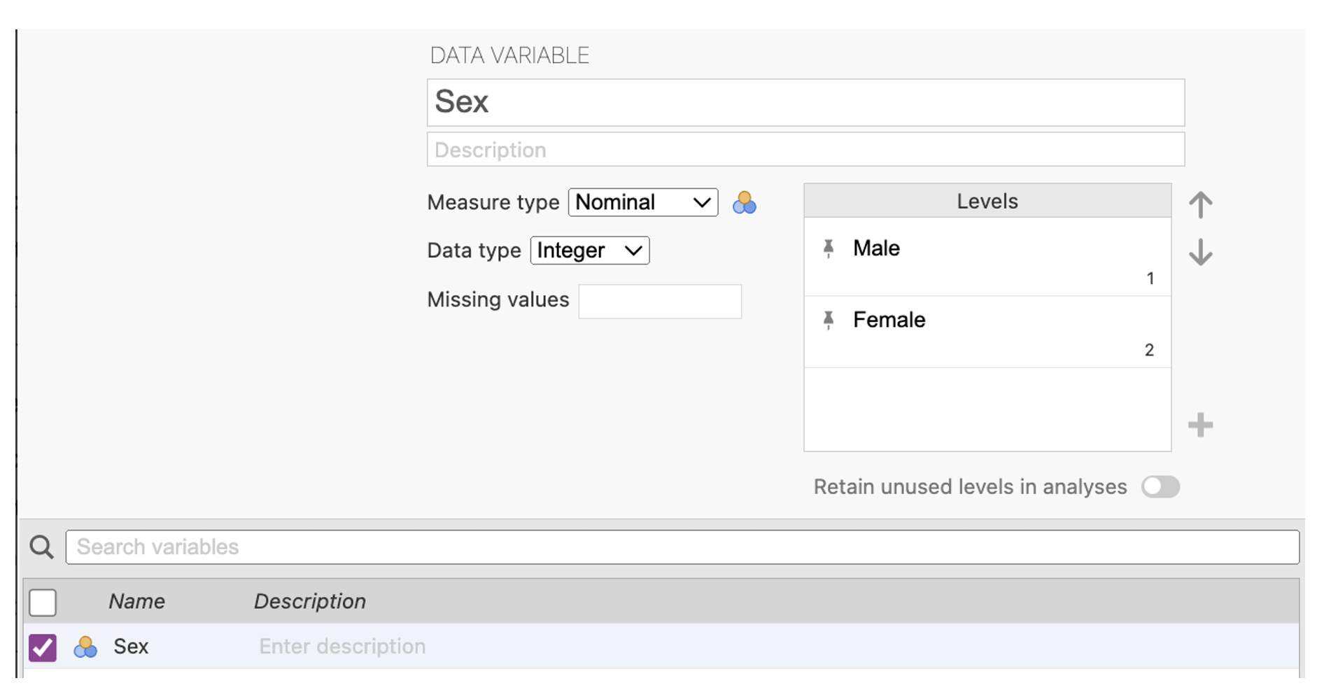 Note. When the levels are created they are pinned and cannot be accidentally deleted. If you type in an extra level and want to remove it, you can click the pin to unpin the level, and then toggle the ‘retain unused levels in analysis’ on and off, which should get rid of it.
4. In the second line of the Variable View, in the Name column, type in the name of the other variable – Dosage.
5. In the edit view again, specify the Measure type as Nominal. In the Levels box you want to specify the dosages of 0 (Zero), 1 (Small), 2 (Moderate), and 3 (Large). The end result should look like the screenshot below (note that the view cuts off the 3 (Large) value and label combination but it is there.
Figure 2.12
Dosage Variable Specification in jamovi
6. Now give the third variable the name of the dependent variable – Performance. In the Edit view denote this variable as continuous. Note that there are no ‘values’ to add for this variable because it is a continuous rather than categorical variable in this study. Categorical variables always need to have their levels specified in terms of value labels, while continuous variables do not.
Figure 2.13
Performance Variable Specification in jamovi

7. Click on the Data tab in the menu ribbon to access the data entry spreadsheet. Click on the first cell. You will notice that a heavy border appears around the first active cell.
Type in the value for sex for the first participant (i.e., either a ‘1’ or a ‘2’ depending on whether they are male or female, respectively), and then use the arrow keys to move right to the next cell. Type in the value of that same participant on drug dosage. Then in the next cell to the right, type in the participant’s maze running performance score.
Use the mouse or arrows to return to the first cell of the next line to enter the second participant’s data.
If you make a mistake, simply highlight the cell where the problem is and type in the correct value. As noted, before you will see that as we type in our data using our numeric values, jamovi will display the value label that corresponds with that numeric value.
If you want to practice saving the jamovi file you can save it to your home drive folder. On the menu bar, click on the three horizontal lines at the far left.
Figure 2.14
Accessing the Main Menu in jamovi

You will then be able to select to save your jamovi file.
Figure 2.15
Saving Data Files in jamovi
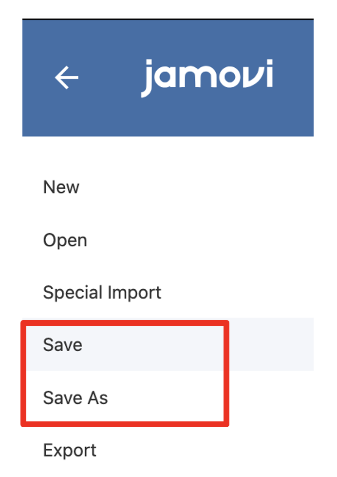
If you are on your own device you can save the file to wherever you choose. If you are in a computer lab on campus navigate to your home H: drive (i.e., the one with your student number).
A Note on Assigning Value Labels
When we have categorical IVs, it doesn’t matter how you label the levels, the results will end up the same. So here we labelled sex as 1 and 2 for males and females, respectively. We could have just as easily (and correctly) assigned them -1 and 1, or 0 and 1. The numbers themselves are meaningless, they are just nominal labels. Likewise, here we assigned the dosage levels values of 0, 1, 2 and 3. However, we could have given them the values of -2, 1.5, 4 and 6. The results of the analysis would be the same. But there are certain conventions to which we generally adhere. Normally, we use whole numbers and start the coding values at 1, or 0 if there is a control group. If there are only two groups, it is also common to code them 1, -1.
Step 2: jamovi for Between Groups Factorial ANOVA
- Select the Analyses menu.
- Click ANOVA, then ANOVA … to open ANOVA analysis menu that allows you to specify a factorial ANOVA.
- Select the dependent variable (i.e., Performance) and then click on the arrow button to move the DV into the Dependent Variable box.
- Select the independent variables in turn (i.e., Sex and Dosage) and click on the arrow button to move each variable into the Fixed Factors box.
- Select Overall model test under Model Fit and select η2 and ϖ2 in the Effect size check boxes
- Click on Model drop down tab. The Sum of squares (bottom right) should be Type 3, which is the default method for partitioning the variance (decomposing sums of squares). With a balanced or orthogonal design, it doesn’t really matter which of the methods you use because the tests of the main effects and interaction are independent – all methods will yield equivalent results.
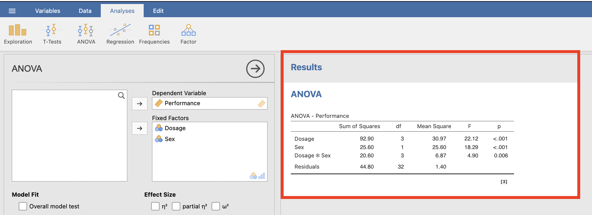
The output of the omnibus tests is displayed below.
Figure 2.16
Omnibus ANOVA Tests in jamovi
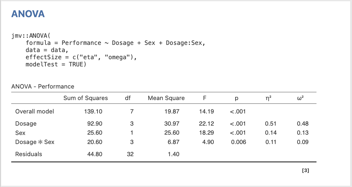
Note that we want means, standard deviations, and confidence intervals for reporting purposes. To get these we need to run a separate descriptives procedure.
If your output above does not have the syntax, you can toggle the syntax on (as described earlier in Activity 2) by clicking on the three dots in top right-hand corner of the jamovi view and ticking ‘syntax mode’ on.
You can also adjust the number of decimal places that jamovi displays. Head to the settings menu which is accessed via the three vertical dots on the far right of the menu ribbon. You will see you have the option to change the number of decimal places (e.g., from 3 to 2 or from 3 to 4) for numbers and (separately) for p values.
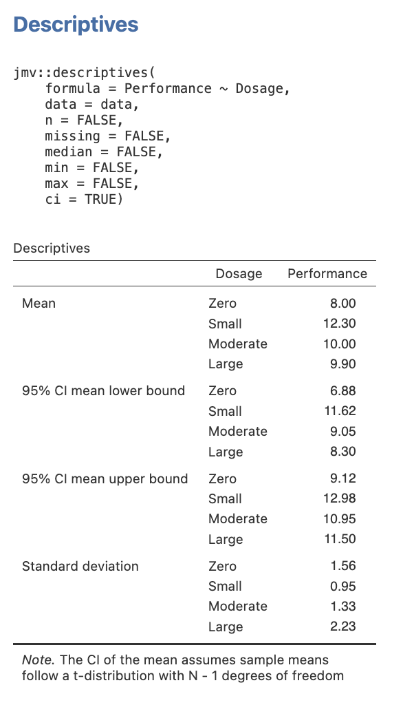
Step 3: Getting Our Cell Means and Standard Deviations in jamovi
Run this twice. Once for Sex and once for Dosage.
- Select the Analyses menu.
- Click Exploration, then Descriptives.
- Select the dependent variable (i.e., Performance) and then click on the arrow button to move the DV into the Variables box.
- Select the independent variables in turn (i.e., Sex and Dosage) and click on the arrow button to move each variable into the Split by box. Click below the output of descriptives for the first IV before doing the second IV, to look at each variable separately.
- In the Statistics drop-down menu ensure that you have the Mean checkbox under the Central Tendency section ticked, and the Std. deviation checkbox under the Dispersion section ticked. Finally, check the Confidence interval for Mean checkbox under Mean Dispersion. You can unselect all other default selections to get a table that has only the means and standard deviations you need.
Here is the table you will get when you follow this process.
Figure 2.17
Descriptive Statistics for Sex in jamovi
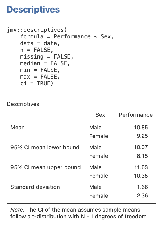
Figure 2.18
Descriptive Statistics for Dosage in jamovi
Note: If you save your data file again now, you will not only save your data but all the analyses you have conducted so far in this exercise. When you go to reopen this data file later on it will have all these analyses saved with it.
Look at the ANOVA table (i.e., ‘ANOVA – performance’ table on the prior page). Copy down the key bits of information here, including the SS (Type III sums of squares), df (degrees of freedom), MS (mean square), F ratios and exact p–values (Sig.).
NB: p-values are to be recorded to three decimal places, while SS, MS and F are to be taken to two. The “Overall model” corresponds to the (Corrected) Total row, and the “Residuals” row corresponds to the Error row.
Table 2.3
Omnibus ANOVA Table for Recording of Results
| Source | SS | df | MS | F | p |
| Sex | |||||
| Dosage | |||||
| Dosage x Sex | |||||
| Error | |||||
| (Corrected) Total |
Note – jamovi refers to the Error row as “Residuals”. The (Corrected) Total needs to be calculated and is the sum of the Residuals row and the Overall Model row.
Go to a version of Table 2.3 formatted for accessibility.
Recall that in previous statistics courses, rather than being given the exact p-values as you are here, you were asked to work out the significance of an F–ratio for yourself. You did this by comparing the obtained F-value from your calculations to the F-critical value found in the F tables (with the appropriate df). In this, if Fobtained was greater than Fcritical, then the result was statistically significant at α = .05. In contrast, if Fobt < Fcrit, then the result was non-significant.
Based on F tables, the Fcrit values for each omnibus test are as below:
Sex: Fα = .05(1, 32) = 4.18
Dosage: Fα = .05(3, 32) = 3.21
Dosage x Sex: Fα = .05(3, 32) = 3.21
Task:
Double-check that your interpretations of significance are the same using exact p-values and the comparison of Fobt to Fcrit.
Write Up the Results for Step 3
Now that you have done the omnibus tests for a two-way between groups factorial ANOVA, state in words what the results mean. That is:
Explain what kind of analysis was done, stating what the IV(s) and the DV were. This includes specifying the levels of the IV(s). Recall that, by convention, we tend to use specific notation to present this information in a condensed manner. Also remember that if this is the first time you have used the term “ANOVA” in the text, this acronym needs to be introduced properly i.e., analysis of variance (ANOVA).
State the significance of the first main effect and describe its direction.
State the significance of the second main effect. NB: note that we don’t describe the direction of effect for this yet, because it involves more than two levels. Hence follow-up tests are required to determine this.
State the significance of the interaction. NB: again, we require follow-up tests to work out what is happening for the interaction before we can describe its direction of effect.
Be sure to include the relevant statistical notation after each of the above omnibus effects (i.e., F, df, p, and η2 or ω2). Note that statistical notation in English/ Latin letters is to be italicised (e.g., F, p), while that in Greek (e.g., η2, ω2) appears as standard text. Further, inferential statistics involving F, and the effect sizes, should be presented to two decimal places, while p-values should go to three.
Be sure to include the relevant marginal or cell means, standard deviations, and 95% confidence intervals when describing the direction of effect. However, if the direction of effect is unknown because follow-up tests are needed to determine this, then hold off presenting these Ms and SDs until you report the follow-up test findings. The number of decimals reported for descriptive statistics (such as means and standard deviations) should be determined by their precision of measurement. In this case, because they were measured as whole numbers in the experiment (i.e., scored 1-15 for maze running performance), they should be taken to only one decimal place for reporting.
*** Your write up is not complete yet. Later in this workbook we will follow-up the significant main effects with more than two levels with main effect comparisons, and we will describe the significant interaction using simple effects and simple comparisons. ***
Test Your Understanding
In ANOVA, we use sums of squares rather than standard deviations as our measure of variance, because we can partition sums of squares into components that reflect each source of variance in turn (i.e., main effects and interactions). Explain how this variance is partitioned in a two-way between groups factorial ANOVA. Hint: use a diagram.
An effect size statistic (e.g., η2) gives the proportion of variance attributable to each effect. In a two-way design, imagine that the main effect of Factor A explained 30% of the variance in the DV, the main effect of Factor B explained 20%, and the AxB interaction explained a further 35%. To what would we attribute the remaining 15%?
Thought Provoker Reading
Chow, S. L. (1988). Significance test or effect size? Psychological Bulletin, 103(1), 105-106. https://doi.org/10.1037/0033-2909.103.1.105
