
8 Activity 8 – Conducting Mixed (Split-Plot) ANOVA using jamovi
Last reviewed 21 February 2025. Current as at jamovi version 2.6.19.
Overview
In this section we look at the analysis of designs involving a combination of within-participants and between group factors. We examine how a mixed (aka split-plot) ANOVA design can be set up and analysed in jamovi. Furthermore, we consider methodological issues with regard to the proper implementation of follow-up comparisons for these designs.
Learning Objectives
- Understand the entering and coding of data in mixed (split-plot) factorial design experiments
- Recognise and be familiar with the jamovi procedures for conducting mixed ANOVA, including interpretation of the associated output
- Comprehend the implementation of appropriate follow-up comparisons for interpreting interactions involving a combination of within-participants and between groups variables
The Overall Model
Mixed factorial designs (sometimes referred to as split-plot designs) are frequently employed in psychological research: these are designs in which you have both one or more between groups IVs and one or more within-participants IVs. The advantage of mixed designs is that you gain power by testing individuals in groups more than once (thereby taking advantage of the strengths of a within-participants design). For example, you might want to test the efficacy of a particular therapy by measuring some state – such as depression – once before therapy begins (to establish a baseline level), and again after the therapy is completed. In many of these kinds of experiments, a second group of people is used, who are also measured at both time points, but who do not receive the therapy (i.e., a control group), creating a between-groups IV (therapy group vs control group). But in the mixed design, you also can test between-groups factors that are unethical to manipulate (e.g., brain damage), as well as IVs that would be confounded or have order effects if you tried to give multiple levels to the same person (e.g., many social norm manipulations).
In the mixed design, participants are nested within the levels of the between groups factor, meaning that each participant is only in one nest (they are either in the control group or in the treatment group). However, participants are crossed with the within-participants factor, i.e., each participant receives all levels of the repeated measures factor. For example, all participants are measured before the intervention [pre] and afterwards [post].
A mixed design represents a combination of the techniques we have used in the between groups and within-participants factorial designs. Recall that the difference between the between groups and within-participants designs lies in the kind of variance we are trying to model and explain. So, to begin with, our mixed model partitions the variance into between- and within-participants variance like this:
Figure 8.1
Partitioning of Variance in Mixed ANOVA
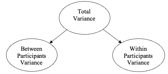
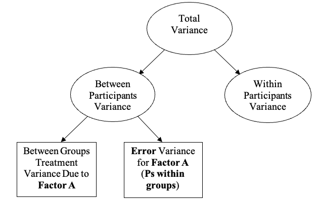
So in the mixed design, we are trying to explain the differences between people’s scores, which has two elements, i.e., the between-participants variance and the within-participants variance. The between-participants variance has two elements of its own: between-groups variance and the within-groups variance. So we partition the between participants component in our mixed model into two further components: the variance due to the treatment, i.e., the variance between groups, versus the variability among participants within each group, which is the error term for the between groups effect. Thus, the model becomes:
Figure 8.2
Partitioning of Between Participants Variance in Mixed ANOVA
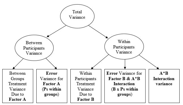
In contrast, for our within-participants IV, we need to look at the within-participants variance. The effect of the within-participants factor represents one component of the within-participants variance, namely the differences among the levels of that factor (in our example, whether there are differences in the average scores on the pre-measure compared to the average scores on the post-measure). The correct error term for this within-participant main effect is the interaction between the within-participants factor B (pre vs post) and the individual differences within the group (i.e., B x Ps within groups). There is a figure for this below.
The third meaningful component of variance is the interaction between the between groups factor and the within participants factor (i.e., the A x B treatment interaction). When we test the interaction, in this example, we are testing whether the difference between the control group and the treatment group, the levels of A, is different between the pre-measure and the post-measure, the two levels of B. The A x B interaction is evaluated using the same error term as the within participants factor B (i.e., B x Ps within groups). Putting this all together, the overall mixed factorial model is:
Figure 8.3
Partitioning of Between Participants and Within Participants Variance in Mixed ANOVA
Simple Effects and Follow-Up Comparisons
Following up significant omnibus effects from a mixed factorial design involves using a different procedure based on which factor/variable is followed up: the between groups IV(s) or the within-participant IV(s). If the main effects are significant and have more than two levels, the main effect comparisons will have different error terms based on whether it is a between or within IV. In addition, to follow up the interaction, we could look at the simple effects of the within participants variable, which involves using a separate error term for each comparison. Alternatively, we could look at the simple effects of the between groups factor, which involves a choice between either using separate error terms for each comparison or using a new error term just for this test, the pooled within-groups error term (i.e., Ps within cells). Because there are a number of different options, it is important to plan ahead as to which tests you will do if needed. The choices of comparisons, simple effects, and simple comparisons ultimately need to be driven by theory and aimed at addressing your hypotheses.
The following study is intended as an exemplar.
Exercise 1: Mixed (Split-Plot) ANOVA in jamovi
The effect of motivation on learning over time in a neuropsychological test
A researcher is interested in the effects of psychological factors on task performance for a test of digit cancellation (which is a neuropsychological test that assesses attention and motor speed). He realises that this is quite a boring task for participants if they have to do it more than once. Performance should improve on the test with an increased number of trials. Yet, as the task is boring, this effect will also depend on how motivated the participant is to improve. The researcher collected data from 12 participants. Each completed the digit cancellation task four times (i.e., there were four trials). However, the participants were randomly allocated to one of three possible motivation conditions. In the low motivation condition, participants were simply told that they would complete the task four times and that they should try their best. In the medium motivation condition, the participants were told that they would complete the task four times, and that they should try their best because they would receive a chocolate bar if their performance improved with each trial. In the high motivation condition, the participants were told that they would complete the task four times, and that they should try their best because they would receive $20 each time their performance improved with each trial. The researcher hypothesised that:
- Overall, there would be an effect of motivation. Specifically, that (a) the medium motivation condition would show better performance than the low condition, and (b) the high motivation condition would show better performance than the medium condition.
- Overall, there would be improvement in performance across the four trials, such that (a) trial 2 would show better performance than trial 1, (b) performance in trial 3 would be better than in trial 2, and (c) that trial 4 would produce better performance than trial 3.
- Motivation would influence the effect of trials. More specifically, the rate of improvement across the trials would be larger in the medium and high motivation conditions than in the low condition.
1. What statistical effects/results would support each of the 3 hypotheses (including relevant follow up tests)?
2. Here is the raw data that you will need to type into jamovi for this exercise
Table 8.1
Number of Digits Cancelled According to Motivation and Trial
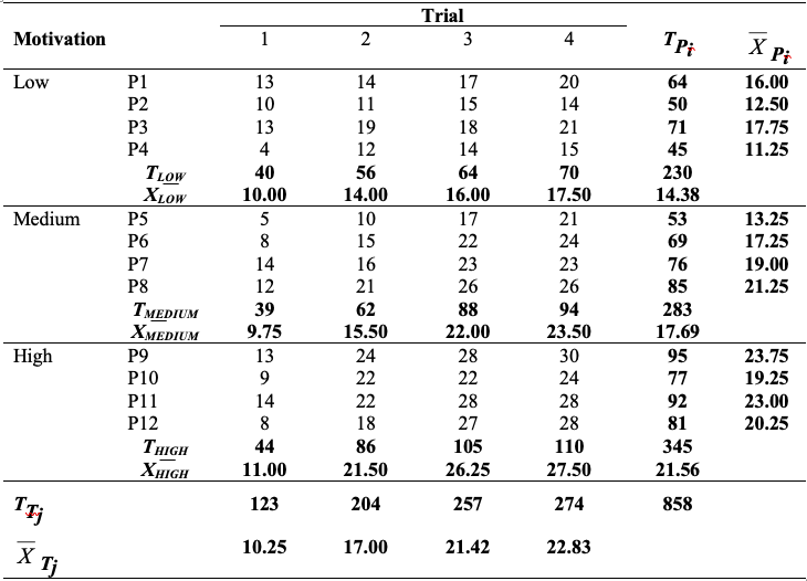
Go to a version of Table 8.1 formatted for accessibility.
Step 1: Enter the Data
- You need 5 columns to enter the data for each participant. The first column will be used to indicate which Motivation group each participant is in. The next four columns will be used to represent the four levels of the within participants factor Trial. So in a mixed design you have one column where you enter the level of the between groups factor, and then additional columns for each level of the within-participants factor. Working in an active jamovi window, click on the Variables tab in the analysis ribbon to define your variables. Type in the first variable name (i.e., Motivation Level) in row A. In the Setup box, define the measure type as Ordinal and enter the Levels ‘low’ ‘medium’ and ‘high’ with codes 1, 2 and 3 in the Levels box.
- Type in the variable names Trial 1, Trial 2, Trial 3 and Trial 4 in the rows underneath Motivation Level in the Variable view.
- Click on the Data tab in the analysis ribbon to enter the data. You will need 12 lines in total (one for each participant).
- Be sure to save your data to a suitable place under an appropriate name.
Alternatively you can download the jamovi file with the data entered already for you. Head to Mixed ANOVA data set.omv and click on the three dots next to the name and then clicking Download. From your computer, open this file up (by double clicking on the ‘.omv’ file if you have jamovi installed directly on your computer, or by starting jamovi and then opening the file). Have a careful look at how the variables have been labelled.
Step 2: jamovi for mixed (split-plot) ANOVA
- Select Analyses -> ANOVA -> Repeated Measures ANOVA.
- In the Repeated Measures Factors box, type in the name of the within-participants factor (i.e., Trials). Give each level the names for the corresponding trials (i.e., Trial 1, Trial 2, Trial 3, and Trial 4).
- Then in the drag each of the four trial variables into their corresponding spots in the Repeated Measures Cells box.
- Select the between groups variable Motivation Level and move this into the Between-Subjects Factor(s) box.
- Under Effect Size tick the box.
- Under Assumption checks ensure Sphericty tests is selected and None, Greenhouse-Geisser, and Huynh-Feldt are selected under Sphericity corrections. (If you were not interested in comparing the GG effect to the other two, you could just tick Greenhouse-Geisser, as this is the adjustment we recommend reporting in all cases, as we have been saying since Activity 7.)
- Under Estimated Marginal Means, move each factor over individually to create a new tem, then select both factors at once and move it over to create a third term in the form of an interaction. Ensure both marginal means plots and marginal means tables are selected under Output.
Step 3: Inspect the output
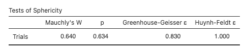
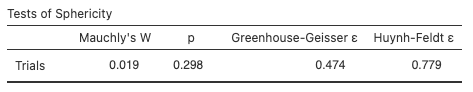
jamovi provides one test of sphericity and one set of epsilon adjustments that can be used to correct the numerator and denominator df of the critical F for both the effect of Trial and the Trial x Motivation interaction (as both involve the “Trial Within-Subjects Effect”). In this example, Mauchly’s Test of Sphericity is NOT SIGNIFICANT (i.e., p = .634, which is p > .05). This means there is no significant violation of the sphericity assumption that this test could detect. We can also see that the Huynh-Feldt epsilon is 1, and the Greenhouse-Geisser epsilon is close to 1. Use of these epsilons to adjust the numerator and denominator df would produce no adjustment in the former case (x 1.000) and only a minor adjustment in the latter (x .830). Because the Mauchly’s test is not robust, we would recommend reporting the GG episilon in all cases.
Figure 8.4
Tests of Sphericity in jamovi
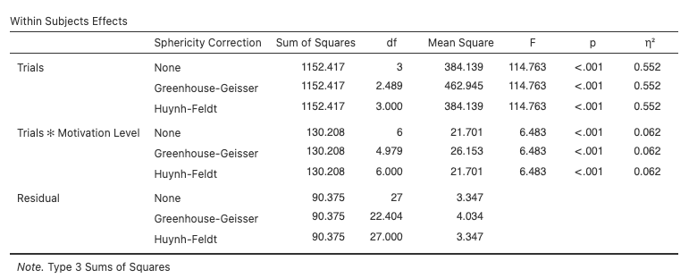
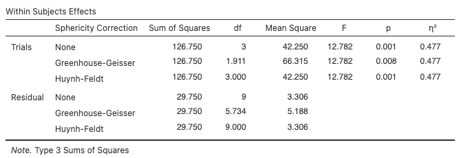
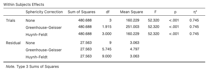
Next you get Tests of Within-Subjects Effects (results for effects involving a within-participants factor, i.e., the main effect of Trial and the Trial x Motivation interaction). These tests are equivalent to the univariate or mixed-model approach to within-participants (repeated measures) designs. Note that the effects of both Trial and Trial x Motivation are tested against the same error term of MST x Ps w/in M (i.e., Trial by Participants nested within Motivation). This error term follows the general principle that the error for a within participants factor consists of an interaction of participants with the treatment effect under consideration. In the mixed (split-plot) design, the only difference is that participants are nested within levels of the between groups factor, so we use the term Ps w/in M rather than just Ps. (As we have remarked above, the Ps variability in the mixed design is divided into the treatment effect, between-group differences for low, medium, and high motivation, and the error term, within-group differences or Ps within groups. Moreover, the Trial x Motivation interaction is evaluated using the same error term as the Trial main effect.
Figure 8.5
Within Subjects Effects in jamovi
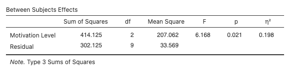
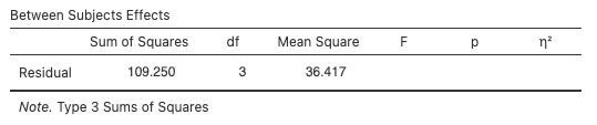
Look at the Tests of Between-Subjects Effects (i.e., the between participants effects). The error term used to test the main effect of Motivation Level in this table is MSPs w/in M. If you compare the mean square error here to the one in the previous table, you can see the error for the test of the between-groups IV is much bigger than the error term for the within-factor and the interaction.
Figure 8.6
Between Subjects Effects in jamovi
Next, examine the marginal and cell means to determine the direction of any significant effects. Just because something is significant does not mean the pattern is in the hypothesised direction.
Figure 8.7
Marginal Means for Trial Main Effect in jamovi
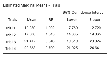
Figure 8.8
Marginal Means for Motivation Main Effect in jamovi
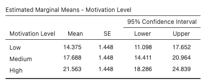
Figure 8.9
Cell Means for Interaction Effect in jamovi
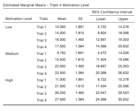
In this case it does look like performance is increasing across the trials, and with higher levels of motivation, but we don’t know whether all of the differences are significant. Depending on the results, we will be needing our main effect comparisons to follow up any significant main effects, and our simple effects and simple comparisons to follow up a significant interaction.
Lastly, inspect the graph. Notice that the lines for the different Motivation levels are not parallel, as represented through the significant Trial x Motivation interaction result.
Figure 8.10
Means Plot for Interaction Effect in jamovi
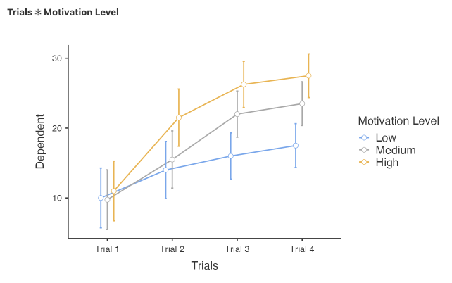
Note. High and low values were calculated as one standard deviation above and below the mean, respectively, for each variable. Error bars represent ±1 standard error (±1SE) from the mean.
Step 4: Fill in the missing details in the Summary Table
| Source | SS | df | MS | F | p |
|---|---|---|---|---|---|
| Between Participants | |||||
| Motivation | |||||
| Ps w/in Motivation | |||||
| Within Participants | |||||
| Trial | |||||
| Trial x Motivation | |||||
| Trial x Ps w/in Motivation | |||||
| Total |
Download Activity 8 Exercise 1 Step 4 (DOCX, 15 KB) to fill in the missing details.
Step 5: jamovi for main effect comparisons in a mixed (split-plot) factorial ANOVA (following up significant main effects)
In order to follow up the significant main effect of Trial (i.e., a within-participants factor with > 2 levels) and/ or Motivation (i.e., a between participants factor with > 2 levels), we need to return to our mixed ANOVA analysis and ask for post hoc tests.
Follow the instructions from before to recreate the main ANOVA model or else click in the ANOVA output in your jamovi output area and this will bring back the analysis and its option choices.
Head to the Post Hoc Tests drop down menu and move motivation across to the right hand box. Then select Trials and move it across also. Under corrections ensure that No correction is selected.
However, if we did not have a priori hypotheses or were performing > 5 comparisons for each set of follow-up tests, we could perform a Bonferroni correction for our comparisons – this is covered in earlier chapters.
Step 6: Inspect the output
Note: A lot of the output will be the same as that given for the omnibus effects, so you’ll need to scroll down (about half-way) to see the new relevant tables below.
First, a reminder of the relevant marginal means for Motivation, which will help you determine the direction of any significant main comparisons found.
Figure 8.11
Marginal Means for Motivation Main Effect in jamovi
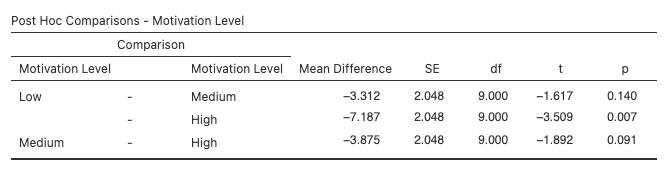
Next let’s look at the Post Hoc comparisons table, which are the main effect comparisons for Motivation. Remember, you should only look at the comparisons relevant to your specific hypotheses. In our case, Hypothesis 1a calls for (1) low vs. medium, and (2) medium vs. high.
Figure 8.12
Post Hoc Tests for Motivation Main Effect in jamovi
Here you are reminded of the relevant marginal means for Trial. These will help determine the direction of effect for any significant main comparisons discovered for Trial.
Figure 8.13
Marginal Means for Trial Main Effect in jamovi
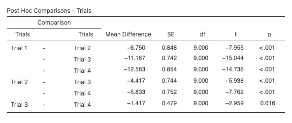
The Posthoc Comparisons provide you with the main effect comparisons for Trial. As stated before, only look at the comparisons relevant to your specific hypotheses. In our case, Hypothesis 2a requires (1) Trial 2 vs. Trial 1; Hypothesis 2b looks to (2) Trial 3 vs. Trial 2, and Hypothesis 2c needs to compare (3) Trial 4 vs. Trial 3.
Figure 8.14
Post Hoc Tests for Trial Main Effect in jamovi
Step 7: jamovi for simple effects and simple comparisons in a mixed (split-plot) factorial ANOVA (following up a significant interaction)
The procedure for conducting simple effects and simple comparisons in a mixed (split-plot) factorial ANOVA depends entirely on your research theory/ hypotheses!
If the theory/ hypotheses suggest the performance of the simple effects of the between groups factor, we would need to run a series of one-way between groups ANOVAs at each level of the within participants factor.
Conversely, if the theory/ hypotheses suggest the need to conduct the simple effects of the within participants factor, we would split the data file by the between groups factor and then run one-way within participants ANOVAs at each level of this between factor.
To determine which set of simple effects is appropriate, let us revisit our third hypothesis:
“Motivation would influence the effect of performance improvement over trials. More specifically, the rate of improvement across the trials would be larger in the medium and high motivation conditions than in the low condition.”
This hypothesis indicates the need to perform the simple effects of Trial (the within participants factor) separately at each level of Motivation (the between groups factor).
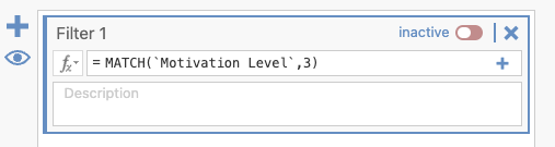
- To achieve this, in the Variables tab, click Filter. In the formula row type in MATCH(‘Motivation Level’,1). This will select just the low motivation group for analysis. We can then edit this filter to say ‘Motivation Level’,2 to get our medium motivation group and “Motivation Level’,3 to get our high motivation group.
- We will want to conduct a one way within-participants ANOVA for each motivation group, which constitutes our simple effects of trial with our above filter set at the three different motivation groups. In other words, to test the simple effects of trial we run three separate one way within-participants ANOVAs here with Trial as the focal IV.
- We can click back into our ANOVA output to bring our analysis and analysis options up. Then move Motivation out of the Between Subjects Factors box to convert the analysis to a one way within-participants ANOVA.
DON’T FORGET! When you have finished conducting these three analyses, remember to turn the split file command off in order to combine the scores back into the original data set. To do this, head back to the Filter you set up and drag the button across from setting it as active to setting it as inactive.
Figure 8.15
Turning Off Filter in jamovi
Step 8: Inspect the output
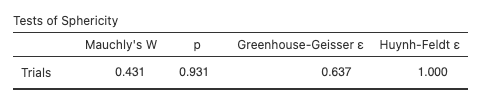
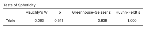
jamovi will provide us with one test of sphericity and one set of epsilon adjustments that can be used to correct the numerator and denominator df of the critical F for each simple effect of trial (i.e., the effect of trial at each level of motivation). This is because each simple effect of trial is essentially a one-way within participants ANOVA, requiring the assumption of sphericity to be tested. Here we see that Mauchly’s Test of Sphericity is NOT SIGNIFICANT for any of the follow up tests (i.e., the simple effect of trial at low, medium and high motivation were p = .931, p = .511, and p = .298, respectively). This means no significant violation of the sphericity assumption occurred, according to the test. We normally report the GG adjustment anyways, because the Mauchly’s test is not robust. Use of the recommended Greenhouse-Geisser epsilon to adjust df would produce moderate corrections to the simple effects of trial at both the low and medium motivation levels (x .637 and x .638, respectively), and a higher adjustment to the simple effect of trial at high motivation (x .474).
Figure 8.16
Tests of Sphericity for Simple Effects of Trial for Low, Medium and High Motivation Level Groups
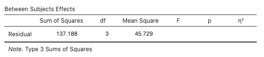
Below is the Tests of Within-Subjects Effects, which are the results for the simple effects of trial. These tests are equivalent to the univariate or mixed-model approach to within-participants (repeated measures) designs. Note that each simple effect test has its own error term, reflecting the fact that each is a one-way within participants ANOVA performed on a separate lot of data (i.e., on the low, medium and high motivation data, respectively). Hence each of these three sub-sets of data have their own unique error.
Figure 8.17
Within Subjects Simple Effects of Trial for Low, Medium and High Motivation Level Groups

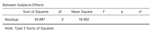
jamovi also provides the Tests of Between-Subjects Effects (i.e., the between participants effects), which in this case is of no particular use to us. Notice that this is divided into three sections, one for each simple effect of trial (at each level of motivation). The error term for each of these represents the variance due to individual differences found in the given sub-sample specific to that simple effect. This information is not typically not reported in psychology, as discussed earlier.
Figure 8.18
Between Subjects Simple Effects of Trial for Low, Medium and High Motivation Level Groups
Next, examine Post Hoc comparisons in conjunction with the cell means to determine the nature and direction of any significant effects. Just because a simple effect is significant and the pattern is as expected, does not mean that all the follow-up tests are significant as well.
Figure 8.19
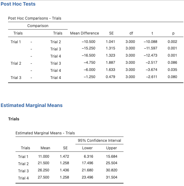
Simple Comparisons and Associated Cell Means for the Simple Effects of Trial for the Low Motivation Level Group
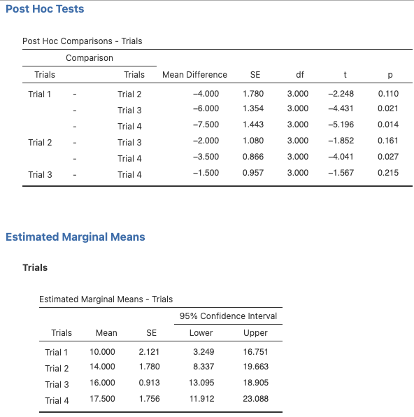
Figure 8.20
Simple Comparisons and Associated Cell Means for the Simple Effects of Trial for the Medium Motivation Level Group
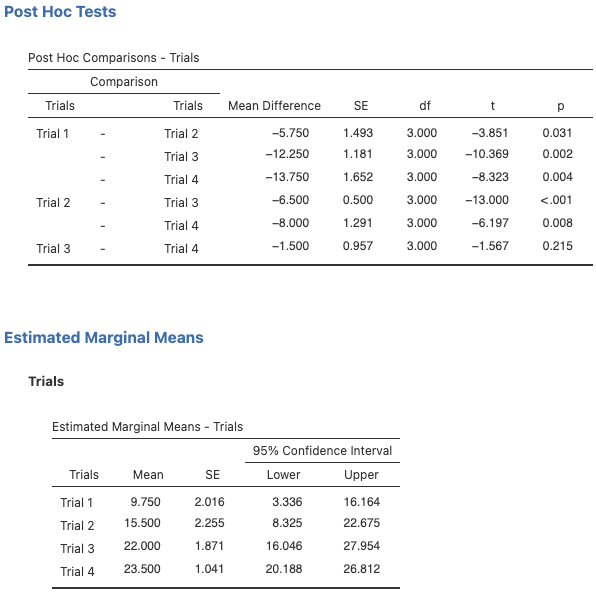
Figure 8.20
Simple Comparisons and Associated Cell Means for the Simple Effects of Trial for the High Motivation Level Group
The Alternative Set of Follow-Up Simple Effects Tests
If the theory/ hypotheses had called for the performance of the simple effects of motivation, we would have conducted a series of one-way between groups ANOVAs exploring the effect of motivation (the between participants factor) at each level of trial. Given the nature of how these variables were entered, we would not need to split the data file beforehand as we did when performing the simple effects of trial (the within-participants factor). Instead, we would simply go ahead and conduct the relevant one-way ANOVAs like this:
- Select Analyses -> ANOVA -> ANOVA. Using the arrow buttons, move Motivation Level (i.e., the between participants factor) into the Fixed Factor(s) box and nominate Trial 1 (the first level of the within participants factor) as the first Dependent Variable.
- This procedure will need to be repeated three times, such that Trial 2, Trial 3 and Trial 4 are entered, in turn, as the Dependent Variable. This will complete the set of four simple effects of motivation, with a one-way between groups ANOVA testing the main effect of motivation at each of the four trial levels.
- If any of these simple effects were found to be significant, since motivation has > 2 levels, simple comparisons would be required to follow up the effect(s). To achieve this, return to the significant simple effect analysis by clicking Analyses -> ANOVA -> ANOVA. Select Post Hoc Tests. Move Motivation Level into the right hand box using the arrow button, and select No correction as the follow-up comparison method under the Correction heading. Remember, you should perform this procedure only as a follow-up for the significant simple effects obtained through the analyses above, and pay attention only to those simple comparisons that address your theory/ hypotheses.
Step 9: Based on the above results, indicate whether each of the researcher’s hypotheses was supported.
Note that there is also the option for “partially supported” if findings are generally in line with the hypothesis, but do not support it fully. Be sure to make use of the relevant marginal and cell means to help determine the correct direction of effect with regard to these.
A reminder of the hypotheses is provided here:
- Overall, there would be an effect of motivation. Specifically, that (a) the medium motivation conditions would show better performance than the low condition, and (b) the high condition would show better performance than the medium condition.
- Overall, there would be improvement in performance across the four trials, such that (a) trial 2 would show better performance than trial 1, (b) performance in trial 3 would be better than in trial 2, and (c) that trial 4 would produce better performance than trial 3.
- Motivation would influence the effect of performance improvement over trials. More specifically, the rate of improvement would be larger in the medium and high motivation conditions than in the low condition.
Click to reveal the answers:
Answers:
Hypothesis 1: Partially Supported
Main effect of motivation found. However, the hypothesised main effect comparisons of low to medium and medium to high motivation did not reach significance. Normally in this case we would also test low to high as an exploratory additional test, which is significant – a weaker pattern than expected.
Hypothesis 2: Supported
Main effect of trial found. Each successive trial was a significant improvement on the previous trial.
Hypothesis 3: Partially Supported
Significant interaction found. All three simple effects significant. In terms of successive trials, the low motivation group did not show significant differences between successive trials (e.g., 1 to 2 and 2 to 3 were not significant, even though 1 to 3 and 2 to 4 were), and the simple effect had the smallest effect size. The medium and high motivation groups both had larger effect sizes than the low motivation groups. However, not all of the increments were significant when the simple effect comparisons are examined.
Recommended Extra Readings
Mixed (or split-plot) ANOVA is covered in many higher-level statistics textbooks – check the Table of Contents to confirm. For example:
Field, A. (2013). Discovering Statistics Using IBM SPSS Statistics: And Sex and Drugs and Rock “N” Roll, 4th Edition. Sage.
Howell, D.C. (2011). Statistical methods for psychology, 8th edition. Wadsworth.
Test Your Understanding
- What is the difference between a two-way Mixed ANOVA and a two-way Within-Participants ANOVA?
- Which main effect will usually have the
largererror term, the test of the between-groups IV or the test of the within-participants IV? What are the implications for power? - If the interaction is significant, which set of simple effects will usually have the smaller error terms? Note. You should plan which set of simple effects you will conduct if the interaction is significant in advance and based on theory.
