
3 Activity 3 – Between Groups Factorial ANOVA: Pairwise Follow-Up Tests in jamovi
Last reviewed 19 December 2024. Current as at jamovi version 2.6.19.
Overview
In this section, we will review how to follow up significant main effects where the factor has more than two levels, using pairwise comparisons in jamovi. We will also learn how to follow up a significant two-way interaction, using simple effects and pairwise simple comparisons.
Learning Objectives
- To illustrate how main effect comparisons (via pairwise t-tests) can be used to examine specific hypotheses about main effects with more than two levels
- To illustrate how simple effects can be used to follow up a significant two-way interaction
- To illustrate how simple comparisons (via pairwise t-tests) can be used to examine specific hypotheses about simple effects containing more than two levels
- To understand when a Bonferroni correction to the αcritical level is appropriate for main effect comparison and simple comparison analyses
- To conduct simple effect analyses in jamovi
- To conduct pairwise main effect comparison and simple comparison analyses in jamovi
- To interpret the output of these follow-up analyses and write up the results
Exercise 5: Follow-up Tests for Main Effects With More Than Two Levels, Applying No Correction to αcritical
Recall the last 4 x 2 experiment in which we found a significant main effect of the drug dosage factor (look back for a reminder of the experimental design). As dosage has four levels (i.e., more than two), the F test for the main effect of dosage does not tell us exactly where the significant difference(s) in performance actually occur between the different drug dosage levels. At this stage, we can only state that the main effect is significant, but we cannot fully address our hypothesis because we cannot yet describe the direction of this effect.
However, you learnt in second-year statistics (in simpler, one-way between groups ANOVA) that when you get a significant F for a factor with more than two levels, the effect can be followed up with linear comparisons/ contrasts and tested for significance with a Bonferroni t’. The same is true in factorial ANOVA, though due to current technology we can now rely on statistical programs to perform most of these follow-up tests for us, rather than calculating them all by hand. This being said, there are three important aspects to recognise when we perform ANOVA follow-up tests in jamovi: (1) we can only easily perform pairwise t-tests in the program (rather than linear contrast t-tests), (2) we do not tend to perform a Bonferroni adjustment to our critical α-level to correct for the number of comparisons made unless it is deemed necessary (see Conservative Follow-Up Tests for Main Effect Comparisons for an overview of when this is recommended), and (3) if a Bonferroni correction is warranted, the jamovi option for performing this does not actually address the Bonferroni adjustment in an appropriate and theoretically meaningful manner. Therefore, the jamovi option should never be used. Instead, a Bonferroni adjustment to the αcritical should be performed by hand (see Conservative Follow-Up Tests for Main Effect Comparisons later where this method is discussed).
In relation to point 1 above, we can follow up significant main effects in a two-way ANOVA using a series of (a) pairwise comparisons, or (b) linear contrasts.
Q: So which do you choose?
A: It depends on your hypotheses.
- If a series of pairwise comparisons will answer your hypotheses, you can conduct these follow-up tests in jamovi.
- If your hypotheses require the comparison of multiple groups in the same contrast, you have to calculate the necessary linear contrasts by hand (download Extra Materials (PDF, 1.14 MB) for how these linear contrast calculations are performed).
Regardless of which technique you choose, be aware that you are performing a two-way between groups ANOVA and so your calculations for the effects of drug dosage will average over the levels of the other factor, in this case, sex. Further, although the statistical technique used may be ‘pairwise t-tests’ or ‘linear contrasts’, because we perform them to follow up a significant main effect, the tests themselves are called ‘main effect comparisons’ or ‘main comparisons’.
Our second hypothesis regarding the main effect of drug dosage was: “a) Overall, rats will perform better when they receive any amount of the drug than when they do not receive the drug. b) However, a small dose will tend to lead to the best performance compared to a large dose.” Hence our second hypothesis does lend itself to investigation via pairwise comparisons through jamovi!
Exercise 5 Task 1
The answer is that there are four pairwise comparisons we really want to perform to address Hypothesis 2. These are:
- zero vs. small drug dosage,
- zero vs. moderate drug dosage,
- zero vs. large drug dosage, and
- small vs. large drug dosage.
The first three comparisons address Hypothesis 2a) regarding the benefits of no drug vs. drug, while the last comparison addresses Hypothesis 2b) with reference to the advantage of a small drug dose over a large dose. Together, these four forms the set of pairwise comparisons necessary to assess our explicit predictions for Hypothesis 2.
***NOTE: If we were to conduct five or more follow-up t–tests (rather than four), we would need to carry out an adjustment to the αcritical level (e.g., employ a Bonferroni correction). This would be because despite being based on a priori hypotheses, there would be five or more comparisons being performed (use Conservative Follow-Up Tests for Main Effect Comparisons, as a guide to when adjustment to the critical α-level is appropriate). Prior to conducting follow-up pairwise t-tests, we always need to check whether an adjustment to the αcritical level is necessary. This will guide our analysis decision regarding whether to employ a Bonferroni correction or not.
Before we execute the actual follow-up main effect comparisons in jamovi, take some time to revisit and eyeball the raw data below. Specifically, look to see whether it is trending in the expected direction for each of our four proposed pairwise comparisons.
Table 3.1
The Effect of Steroidal Dosage and Sex on Maze Running Performance in Rats
|
Dosage |
Sex |
MDi |
|
|
|
Male |
Female |
|
|
Zero |
10 10 8 10 7 M11 = 9.0 |
6 7 6 8 8 M12 = 7.0 |
8.0 |
|
Small |
10 13 13 12 12 M21 = 12.0 |
12 13 13 12 13 M22 = 12.6 |
12.3 |
|
Moderate |
12 10 12 11 9 M31 = 10.8 |
9 9 10 8 10 M32 = 9.2 |
10.0 |
|
Large |
10 11 12 12 13 M41 = 11.6 |
9 10 6 9 7 M42 = 8.2 |
9.9 |
|
MSj |
10.9 |
9.3 |
10.1 |
Go to a version of Table 3.1 formatted for accessibility.
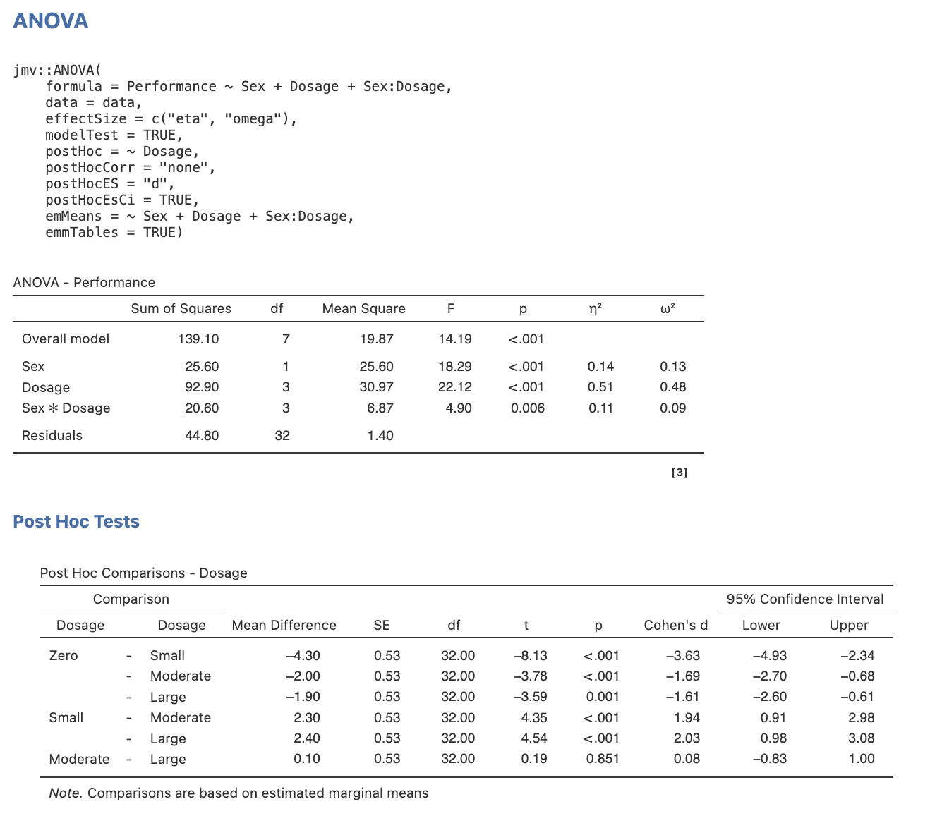
jamovi For Main Effect Comparisons With No Correction To αcritical
As a reminder, we are performing main effect comparisons to follow up the significant main effect of drug dosage (a factor with more than two levels) using pairwise t-tests with no correction to our critical α-level (i.e., no Bonferroni adjustment).
- If our hypotheses had required the use of linear contrasts (rather than pairwise comparisons) as the means of follow-up, we would have needed to perform these calculations by hand.
- Also remember that although we are conducting our main effect comparisons here with no correction to αcritical, if (a) these comparisons had not been based on our predictions, (b) our number of comparisons performed had been five or more, and/ or (c) these analyses were being performed on an overly large dataset or were grounded in weak theory, then we would adjust the αcritical level. We will demonstrate how to perform main comparisons with a Bonferroni correction to the critical α-level later in Exercise 6.
Let’s have a go at conducting main effect comparisons in jamovi.
Step 1: Open the Data File
Since we entered the data last time, you just need to open up the data file in jamovi. Here is the data file again in case you need it – Factorial BG ANOVA data file.omv (click on the three dots and select download). If you saved the data file on your computer at the end of the previous exercise you will have your analysis and menu options also saved with it. If you need to recreate the analysis the steps are outlined in full below. If the analysis has been saved with your data, click in the ANOVA output in the results view and you will see the ANOVA menu appear on the left side with your previously selected options and you can just select the extra options.
Step 2: jamovi for Pairwise Main Effect Comparisons in Between Groups Factorial ANOVA
- Select the Analyses menu.
- Click ANOVA, then ANOVA … to open ANOVA analysis menu that allows you to specify a factorial ANOVA.
- Select the dependent variable (i.e., Performance) and then click on the arrow button to move the DV into the Dependent Variable box.
- Select the independent variables in turn (i.e., Sex and Dosage) and click on the arrow button to move each variable into the Fixed Factors box.
- Select Overall model test under Model Fit and select η2 and ϖ2 in the Effect size check boxes
- Click on the Model drop-down tab. The Sum of squares (bottom right) should be Type 3, which is the default method for partitioning the variance (decomposing sums of squares). With a balanced or orthogonal design, it doesn’t really matter which of the methods you use because the tests of the main effects and interaction are independent – all methods will yield equivalent results.
- NEW STEP: Under the Post Hoc Tests drop-down tab select Dosage in the listing to the left and click the arrow to add it to the box on the right. Under Correction tick the “No Correction” checkbox and ensure that other options are not selected. Under Effect Size tick the Cohen’s d checkbox along with Confidence interval which will be set at 95% as a default.
Step 3: Examine the Output
Task 1
Take a look at the output, paying special attention to the main effect comparisons. Note what pieces of information are present and which are missing.
Omnibus ANOVA and Main Effect Comparisons for Dosage
 Note. In the settings menu for jamovi (which you can access by clicking the three vertical dots on the far right of the jamovi menu ribbon) you can change the number of decimal places in your output for p values as well as numbers. APA 7 format suggests that p values be reported to 3 decimal places, and inferential statistics (e.g., t) are reported to 2. You also can request the means within ANOVA using the emMeans function – but it is more straightforward using the commands below.
Getting Our Marginal Means and Standard Deviations in jamovi
- Select the Analyses menu.
- Click Exploration, then Descriptives.
- Select the dependent variable (i.e., Performance) and then click on the arrow button to move the DV into the Variables box.
- Select the independent variables for our main effect (i.e., Dosage) and click on the arrow button to move each variable into the Split by box.
- In the Statistics drop-down menu ensure that you have the Mean checkbox under the Central Tendency section ticked, and the Std. deviation checkbox under the Dispersion section ticked. Finally, check the Confidence interval for Mean checkbox under Mean Dispersion. You can unselect all other default selections to get a table that has only the means and standard deviations you need.
Here is the table you will get when you follow this process.
Figure 3.2
Descriptive Statistics for the Main Effect of Dosage
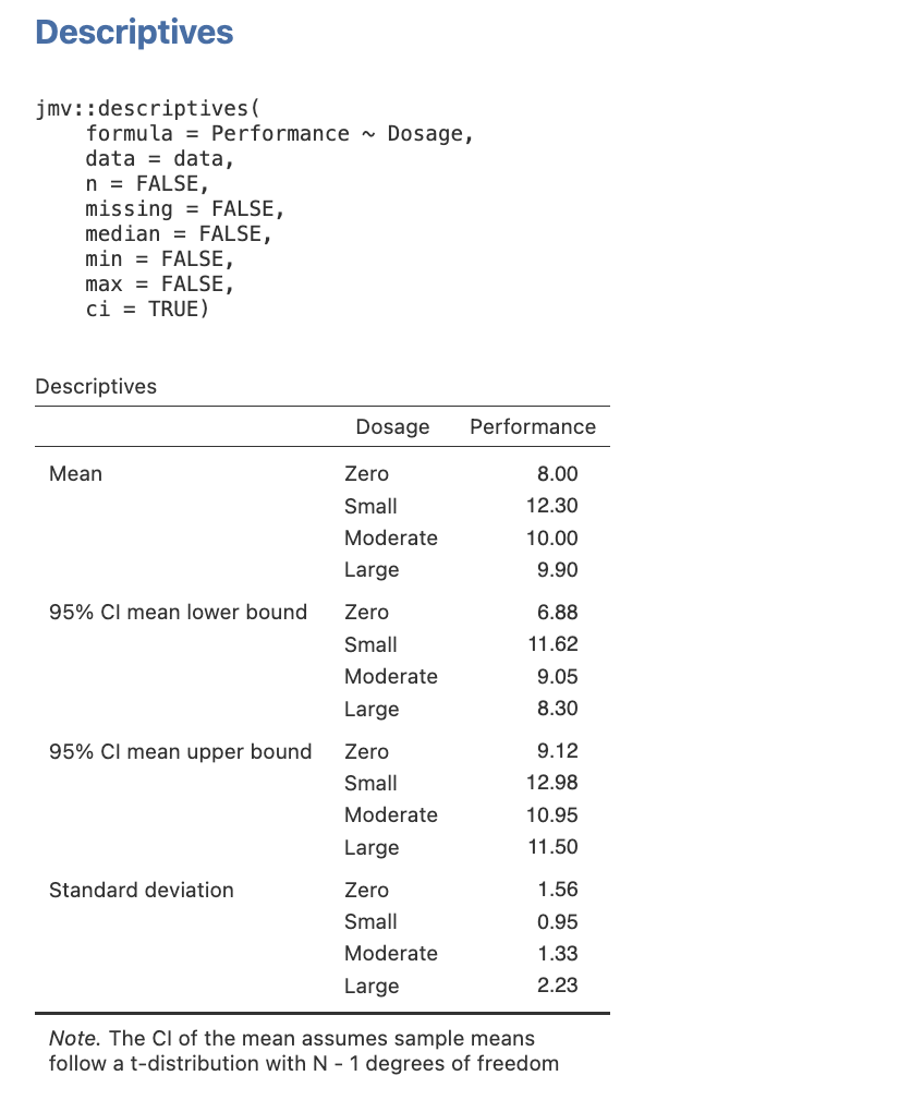
Task 2
- Determine which of our four focal pairwise comparisons were significant, and
- For those comparisons that were identified as significant, revisit the marginal means to determine their direction of effect (e.g., identify the larger mean for each).
Task 3
Write in words what the findings mean as you would in a Results section.
That is, report:
- The overall type of analysis that was performed, stating what the IV(s) and DV were. This includes specifying the levels of the IV(s). Again, recall that by convention, we tend to use specific notation to present this information in a condensed manner.
- The main effect of drug dosage, stating its significance.
- Then, report the main effect comparisons (stating the significance and direction for each).
Don’t forget to include relevant:
- Statistical notation after the omnibus test (i.e., F, df, p, η2 or ω2).
- Statistical notation after each main effect comparison (i.e., t, df, p, d).
- Marginal means and standard deviations when describing the direction of effect. NB: These statistics are only reported once each and not repeated i.e., they are given the first time the relevant group is mentioned in the text.
- Information about the type of main comparisons that were performed, including:
- Whether they were pairwise t-tests or linear contrasts,
- The number of comparisons conducted,
- The critical α-level employed for each comparison, and
- What type of correction was used (NB: if no adjustment to the critical α-level was performed, this last piece of information is typically omitted).
As a reminder:
- Statistical notation in English/ Latin letters needs to be italicised (e.g., F, t, p, d), while that in Greek (e.g., η2, ω2) appears as standard text. Likewise, notation for subscripts and superscripts are presented in standard text (i.e., these do not appear in italics).
- Inferential statistics (e.g., F, t), effect sizes (e.g., η2, ω2, d) and confidence intervals should be presented to two decimal places, while p-values go to three.
- Descriptive statistics (such as means and standard deviations) are given to the number of decimals suited to their precision of measurement. In our case, maze running performance was scored as whole numbers (i.e., scaled 1-15). Therefore, descriptive statistics regarding the means and standard deviations for this should be taken to one decimal place for reporting.
- Any value that happens to be very small but can potentially exceed a threshold of ±1 (e.g., M, SD, F, t, d), should have a 0 preceding the decimal point. However, any value that cannot potentially exceed ±1 (e.g., p, η2, ω2), should not have a 0 before the decimal.
- The direction of effect for main comparisons should also be reflected in the positive or negative valence of the reported t-value. That is, a positive t-value indicates that the first reported group involved in the comparison had a higher mean than the second group. In contrast, a negative t-value indicates that the first reported group involved in the comparison had a lower mean than the second group.
- The jamovi output above gives the CIs for the means, and when the CIs for two means do not overlap, we interpret the difference as significant. The jamovi output for the t-tests also gives CIs, but for the effect size measure, d. If you are not troubled by limitations regarding your word count, you can comprehensively report CIs for all of the various parameters reported (and in some other software you would also get CIs for the t and report that too). However, if you are trying to write tersely, the CIs for the effect sizes are the most conventional to prioritise including.
*** You have not yet finished all the follow-up tests. More are needed in order to decompose the significant interaction (i.e., simple effects and simple comparisons). These will be covered in Exercises 7 and 8. ***
Exercise 6: Follow-up Tests for Main Effects With More Than Two Levels, Applying a Bonferroni Correction to αcritical
Conservative Follow-Up Tests for Main Effect Comparisons
In the jamovi exercise above, we followed up our significant main effect of drug dosage (i.e., a factor with more than two levels) using a series of pairwise t-tests where no correction to αcritical was made for the number of comparisons performed. There are some circumstances when it is more appropriate to use a Bonferroni correction for this. The Bonferroni procedure adjusts the critical value to which we compare our t-test statistic, maintaining the overall familywise error rate at α = .05 (or α = .01). It does this by taking the critical α-level of .05 and dividing it by the number of comparisons being made. For example, ten follow-up comparisons would make use of a critical significance level of α = .005 each (i.e., α = .05 / 10). This, in turn, makes the t-critical value more conservative (i.e., larger) and thus more difficult for our t-obtained value to exceed in order to be considered significant.
The advantage of applying a Bonferroni correction to follow-up tests is that it ensures no inflation of our familywise error rate. To illustrate, hypothetically let’s say we had five (rather than four) comparisons, where we also wanted to look at the effect of small versus moderate dosage. Consider what would happen if we performed these five comparisons without correction, each at α = .05. Our familywise error rate for these would be a whacking great α = .250 (i.e., α = .05 x 5)! Yet if we applied a Bonferroni adjustment to αcritical based on these same five follow-up tests, familywise error would remain at α = .05 (where each comparison would be evaluated against a new αcritical of .05 / 5 = .01). To identify the use of a Bonferroni correction in a write-up, the author(s) should explicitly state that a Bonferroni correction was used for [number of] comparisons, where familywise error rate was maintained at α = .05 or where each comparison was evaluated against α = [.05 / number of comparisons], and change the statistical notation from t to t’ (note the addition of the apostrophe/ prime sign).
When to Apply a Bonferroni Correction to the Critical α-level
The decision of whether or not to employ a Bonferroni correction to αcritical for follow-up comparison t-tests rests on the answers to three major questions. These are:
1. Were my predictions for these comparisons made post hoc?
A priori predictions are those made before data collection and analysis, and are based upon theory. In contrast, post hoc comparisons are more exploratory and are performed after initial data analysis, when an unexpected result emerges (e.g., significant main or simple effect involving a factor with more than two levels) and we wish to determine where the difference(s) between groups lies. Hence, post hoc comparisons are not planned and generally not grounded in appropriate theory. In such cases, performing a correction to the critical α-level for our t-tests is a prudent option.
2. Am I performing five or more comparisons?
Follow-up comparisons numbering five or more drastically boost our familywise error rate because – as stated above – each comparison carries with it an α-level of .05. Therefore, our total error rate for a series of follow-up comparisons is .05 multiplied by the number of comparisons being made. This means that our chances of making a Type I error (i.e., claiming a result to be significant when in reality there is no genuine relationship) are also dramatically increased. So whenever we are performing five or more comparisons to follow-up a single significant main (or simple) effect, the familywise error rate is considered too great and an adjustment to our αcritical is needed.
3. Do I want to be conservative?
Times when we want to adopt a conservative approach are cases where (a) the data set we are working with is overly large (e.g., observations numbering in the hundreds to thousands), and/ or (b) the research area is novel and therefore, our theory driving predictions is weak or exploratory. If either of these conditions is not present, however, there is no real need for us to be conservative and adjust αcritical for the follow-up t-tests.
In a nutshell, if you answer “yes” to any of the above three questions, then a Bonferroni adjustment to the critical α-level for your follow-up t-tests should be employed! However, if you answer “no” to all three, then a Bonferroni correction is not warranted.
Having said this, some researchers may still err on the side of caution and adjust the αcritical regardless of their answers to the previous questions. Yet although there may be the desire to always be conservative, we must consider the potential disadvantages of doing so. In psychology, a Bonferroni adjustment is often seen to be a bit too conservative to apply as standard practice (i.e., it should only be applied as required, following the above guidelines). Specifically, although a Bonferroni correction to αcritical is acknowledged to protect against the danger of overclaiming differences between groups as being significant, it does so at the cost of potentially underclaiming these results. As a consequence, we may miss out on detecting important and genuine relationships. That is, by overcompensating for a Type I error, we risk a problem of Type II error.
In the previous activity, you were asked to identify the series of pairwise comparisons that would be required to address Hypothesis 2a and 2b of the Dosage x Sex study. These were:
- zero vs. small drug dosage,
- zero vs. moderate drug dosage,
- zero vs. large drug dosage, and
- small vs. large drug dosage.
Therefore, a Bonferroni correction to our critical α-level is NOT recommended because we are only conducting four follow-up main effect comparisons for drug dosage in line with our a priori study predictions, on a small data set in a research area that is not novel (thus answering “no” to all three questions regarding when to employ a Bonferroni correction). However, when a Bonferroni adjustment to the critical α for follow-up comparisons is warranted, we can conduct the vast majority of this procedure through jamovi, following the steps we completed earlier in Exercise 5. However, an additional two steps are required at the end. These involve (1) a simple hand calculation to determine the new Bonferroni adjusted critical α-level, and (2) a series of visual comparisons between this new critical α-level cut-off and the p-values obtained in jamovi for each comparison, in order to determine significance/ non-significance. [Note again that all this only applies when pairwise comparisons are appropriate to follow up the research hypotheses – linear contrasts would need to be calculated fully by hand].
jamovi for Main Effect Comparisons With a Bonferroni Correction to αcritical
As stated before, the application of a Bonferroni adjustment to our critical α-level is achieved through an additional two steps to those outlined above in Exercise 5 (which involved the use of no correction to αcritical through the No correction option). These extra steps which occur at the end – making up a new step 4 and 5 – are:
4. Determine the number of comparisons in which you are interested (i.e., upon which the Bonferroni adjustment to αcritical will be based). This should be dictated by your hypotheses. Therefore, it may involve all or only a subset of all the possible pairwise comparison combinations. Divide your familywise error rate of αFW = .05 by this number in order to ascertain the new critical α-level cut-off value. In the hypothetical case given earlier (where we also wanted to explore the effect of small vs. moderate dosage), we had five comparisons in which we were interested. Hence, we would re-calculate our new critical cut-off value to be α = .05 / 5 = .01. This means that each comparison will now be evaluated against α = .01 rather than α = .05. Thus, in total, the familywise error rate across the five comparisons will be maintained at α = .05 (i.e., α = .01 x 5 comparisons).
Note: When calculating a Bonferroni corrected critical α-level, it is standard practice to round this value to three decimal places. This allows for an easy comparison between this critical cut-off and the significance values in jamovi (i.e., p-values, which also appear rounded to three decimals in the table display). Furthermore, rounding of these figures to three decimal places also adheres to APA guidelines regarding reporting of p-values (which appear to three decimals) and α-levels (which appear up to three decimals) in a write-up.
5. Locate the main effect comparisons table in the jamovi output (labelled Post Hoc Comparisons – Dosage in the Post Hoc Tests section), and find the significance level (p-value) for each of the five new hypothetical focal comparisons. Compare each to the new Bonferroni adjusted critical value (i.e., α = .01) in order to determine whether each is significant or non-significant. Here, any comparison with p < .01 is considered significant, while those with p ≥ .01 are non-significant. The significance (i.e., p-value) for each of the five new key main comparisons is now evaluated against our Bonferroni critical α = .01 (rather than our usual α = .05) in order to determine whether each is significant or non-significant.
Figure 3.3
Jamovi Main Effect Comparisons for the Dosage Main Effect
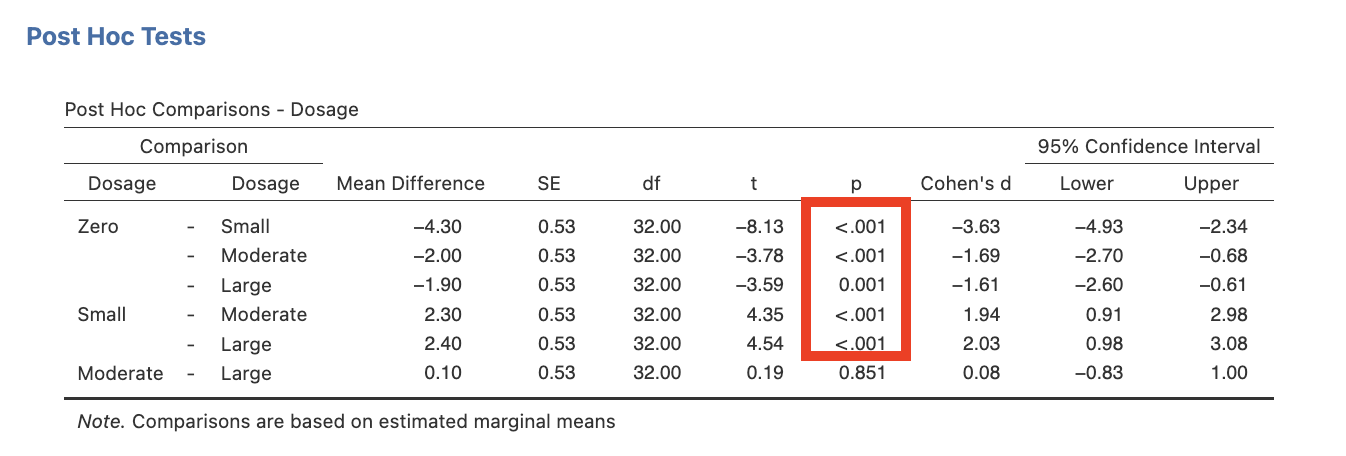
Task 1
Based on the above steps, look at the main effect comparisons in the Post hoc Comparisons table in Figure 3.1 (this is from your earlier analysis involving no correction to αcritical via the LSD adjustment method). Apply a Bonferroni correction to our αcritical and use this to assess each of the new five hypothetical key comparisons.
In the space below (a) state whether or not each of these five comparisons was significant, (b) for the significant comparisons, determine their direction of effect (hint: revisit the marginal means to help with this), and (c) provide the t value, and Cohen’s d effect size for each.
Cool Trick in jamovi
Sometimes the α-level we calculate as our Bonferroni critical cut-off is not as neat and clean as α = .01. Sometimes it has a long string of decimals which, although we could round to three decimal places (as per APA guidelines), would result in the loss of some accuracy. Normally this isn’t a problem. However, there are rare cases when this could make the difference between concluding that a comparison is significant versus non-significant. At such times, some researchers prefer to use a method that allows them to gain more accurate significance values for their comparisons and therefore, facilitates more accurate conclusions regarding the significance/ non-significance of these as compared to αcritical. This method is outlined below:
For greater accuracy regarding p-values in jamovi, head to the settings menu accessed via the three vertical dots on the far right of the menu ribbon. You will see you have the option to increase the number of decimal places for p values. Increase this to 4 or 5. You should now be able to determine more easily if each of your comparisons is significant or non-significant, as compared to your Bonferroni adjusted critical α-level (taken to as many decimals as is appropriate).
All this being said, recall that APA standards for writing state that p-values are to be reported to three decimal places, and critical α-levels to no more than three decimals. Hence, it is more conservative that if – when rounded to three decimals – the p-value for a main/ simple comparison and the Bonferroni critical α-level are the same, then this result should be concluded to be “marginally significant”, and interpreted as such in the Discussion.
Just Out of Curiosity, Why Don’t We Use the Bonferroni Correction Option in jamovi?
Although jamovi offers a Bonferroni correction option for follow-up comparisons that would be far easier for us to use than the method in Exercise 6, we refrain from employing this because it has two major flaws. The first is that it approaches the adjustment to αcritical in a way that is inconsistent with the theory underlying the Bonferroni correction. The second is that it assumes an adjustment for all possible pairwise comparison combinations, when in actual fact most times we only wish to adjust for a subset of these (i.e., only those relevant to our hypotheses). Each of these points is expanded upon in more detail below.
jamovi Bonferroni Option Flaw 1:
Recall that theoretically, a Bonferroni correction aims to take our familywise error rate of
αFW = .05 and adjust this critical value based on the number of tests being performed. Specifically, it divides αFW = .05 by the number of comparisons being conducted. This results in a more conservative critical α-level cut-off that is harder for each comparison’s t-test statistic to exceed. It also maintains the total or familywise error rate at α = .05 across all the comparisons being made. In our new hypothetical case, we wanted to perform five main comparisons to follow-up our significant drug dosage main effect, so our new critical α-level became α = .05 / 5 = .01. Hence the p-values for each of our five comparisons would not be evaluated for significance against α = .05, but rather against the stricter Bonferroni corrected α = .01 criterion.
The key concept to take note of here is that a Bonferroni adjustment alters the critical α-level against which we evaluate our comparison’s significance level (i.e., p-value, as reported in jamovi). At no stage do we aim to alter the comparison significance levels themselves, as to do so would suggest that the probability of that comparison result occurring in the sample has somehow altered (when in actual fact it should not)! To reiterate, the logic behind the Bonferroni correction is that the significance level for a main/ simple comparison in a sample (as seen by its p-value reported in jamovi) should not change, only the critical α cut-off criteria against which we compare it to determine whether or not it is considered significant. The degree of how conservative we make this new critical cut-off is in proportion to how many comparisons we conduct, hence why we divide αFW = .05 by the number of comparisons made.
In stark contrast to this, the jamovi option for the Bonferroni correction produces results which adjust the given significance levels of our sample comparisons (i.e., the reported p-values themselves – which in reality should not change)! How jamovi goes about this is to take the original reported significance level, and weight (i.e., multiply) it by the number of pairwise comparisons. This weighted p-value is then interpreted against a critical cut-off of α = .05. This would – strangely enough – lead us to the same conclusions as those when we apply the proper method for the Bonferroni correction. However, keep in mind that what has been created here are now arbitrary and inflated p-values that no longer accurately represent the likelihoods of achieving those particular main/ simple comparison results in the sample if the null hypothesis is true! So the p-values jamovi generates through its Bonferroni correction option are not correct as applied to these comparisons and should not be reported in a write-up under any circumstances.
jamovi Bonferroni Option Flaw 2:
Another key issue with the jamovi procedure for the Bonferroni adjustment is that it corrects for all possible pairwise comparison combinations among our variable levels. It does not have an option for only correcting for a subset of these. Therefore, the p-value results produced will be even more inaccurate and misleading if we are not interested in all of the pairwise comparisons in the set (as guided by our hypotheses)! This is because the inappropriate weighting of the original reported significance levels for each comparison is done by the number of all possible pairwise combinations, not just the ones in which we’re interested. That is, the original accurate p-values are multiplied by the total number of pairwise comparisons possible in the set. So you can see how this would compound the first problem regarding the inappropriate weighting of the reported p-values in the first place! Further, we can no longer even compare these p-values to α = .05 to determine their significance/ non-significance in instances where we are not interested in all the pairwise combinations.
Let’s have a look at how these problems play out with regard to our current hypothetical set of five required comparisons…
WARNING: The following exercise involving the performance of a Bonferroni correction through jamovi is for illustrative purposes only and should not be employed in any statistical analyses you may conduct, because of the two flaws noted above!
To apply a Bonferroni correction in Jamovi the instructions from Exercise 5 involving no correction to αcritical would only change for Step 5, making it:
5. Click on the Post Hoc drop-down list. Move Dosage into the right side box. Under Correction tick the “Bonferroni” check box.
The output would remain almost the same as before, with only the last table changing. This table would now present as:
Figure 3.4
Bonferroni Adjusted Main Effect Comparisons in jamovi
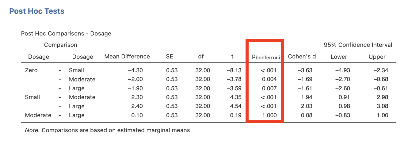
Notice the changes to the reported significance levels (i.e., p-values) for each comparison in the jamovi output. These adjusted p-values can now be compared to α = .05 for significance. HOWEVER, remember that these values have been artificially inflated and no longer represent the probability of finding these results in our sample if the null hypothesis is true!
Comparing this table to Figure 3.1 produced using the No correction option (i.e., no correction to αcritical), we see that the p-values generated here are weighted by six, which is the total number of pairwise comparisons possible amongst the four levels of drug dosage (i.e., zero vs. small, zero vs. moderate, zero vs. large, small vs. moderate, small vs. large, and moderate vs. large – the latter one of which was not relevant to our new hypothetical predictions). Therefore, each of the reported p-values given here is six times larger than they are in the actual sample! Note that some inconsistency in figures may occur due to jamovi rounding for the original no correction p-values before they were multiplied by the full number of pairwise comparisons to obtain the Bonferroni adjusted p-values, as well as rounding after this calculation. Also be aware that values above 1.00 were rounded down to 1.00, because p cannot exceed 1. Just as the no correction p-values can be too liberal with many comparisons (resulting in Type I error), the Bonferroni p-values produced through jamovi can be too conservative (resulting in Type II error).
So, in sum, the jamovi Bonferroni option should be avoided for two major reasons:
- It alters the reported significance levels for our obtained comparisons, which should not change. Thus this option provides inaccurate and misleading p-values for our sample, and
- It makes adjustments based on all possible pairwise comparison combinations, not just the ones that interest us according to our hypotheses.
This is why we opt for performing the Bonferroni correction to our αcritical by hand instead!
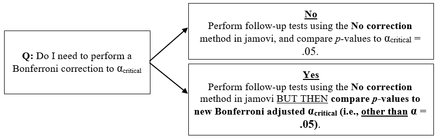
The Decision Tree
The following represents a brief decision tree that can help you choose how best to approach the use (or non-use) of the Bonferroni correction to your αcritical for follow-up comparisons.
Figure 3.5
Decision Tree for Decision Marking regarding Bonferroni Corrections
Reporting Comparisons that Employed a Bonferroni Correction
When writing up the results of main (or simple) effect comparisons that employed a Bonferroni adjustment to the αcritical level, we must be sure to:
- Clearly state that a Bonferroni adjustment was used,
- Explain that the main/ simple comparisons were performed to follow-up the significant main/ simple effect of Factor X,
- Report the number of comparisons performed,
- Provide the Bonferroni adjusted critical α-level used (whether for the overall familywise error rate or for each comparison), and
- Then, for each comparison, report the significance and direction of effect.
The first four steps often are reported concisely along the lines of “The significant main effect of drug dosage was followed up with a series of pairwise t-tests, using a Bonferroni correction for five main comparisons where familywise error rate was maintained at α =.05.” OR “Pairwise main comparisons were performed to follow up this significant effect, using a Bonferroni correction where each of the five comparisons was evaluated against α =.01.”
Interaction Follow Up Tests
Continuing with the Drug Dosage x Sex example, recall that this experiment used a 4 (drug dosage: zero, small, moderate, large) x 2 (sex: male, female) between groups factorial design. We will need to follow up the significant interaction with simple effects (Exercise 7) AND – if we perform simple effects on a factor with more than two levels (and if any of these turn out to be significant) – then we will have to further follow up these significant simple effects with simple comparisons (Exercise 8).
Simple Effects
Let’s look again at the data with which we’ve been working. We have a significant interaction, and need to describe it in order to fully address our third hypothesis.
Table 3.2
Omnibus ANOVA results for the Effect of Steroidal Dosage and Sex on Maze Running Performance in Rats
|
Source |
SS |
df |
MS |
F |
p |
|
Sex |
25.60 |
1 |
25.60 |
18.29 |
< .001 |
|
Dosage |
92.90 |
3 |
30.97 |
22.12 |
< .001 |
|
Dosage x Sex |
20.60 |
3 |
6.87 |
4.90 |
.006 |
|
Error |
44.80 |
32 |
1.40 |
|
|
|
(Corrected) Total |
183.90 |
39 |
|
|
|
Go to a version of Table 3.2 formatted for accessibility.
Remember, our third hypothesis was that:
“The effect of drug dosage will differ for males compared to females. While both sexes will exhibit increased performance when they receive any amount of the drug than when they do not, the particular benefits of the small drug dosage (compared to the large dose) will be more noticeable in female rats than in male rats.”
Before we can do anything to follow up our significant interaction, we must figure out exactly which follow up tests we want to do. Hypothesis 3 specifically refers to a certain set of simple effects. To which set of simple effects does this hypothesis refer?
So we will have one simple effect of drug dosage for when the rats are female, and another simple effect of drug dosage for when the rats are male.
Now we will perform this analysis in jamovi.
Exercise 7: Follow-Up Tests for an Interaction
Simple Effects in jamovi
Below is the data from the Drug Dosage x Sex experiment again:
Table 3.3
The Effect of Steroidal Dosage and Sex on Maze Running Performance in Rats
|
Dosage |
Sex |
|
|
|
Male |
Female |
|
Zero |
10 10 8 10 7 |
6 7 6 8 8 |
|
Small |
10 13 13 12 12 |
12 13 13 12 13 |
|
Moderate |
12 10 12 11 9 |
9 9 10 8 10 |
|
Large |
10 11 12 12 13 |
9 10 6 9 7 |
Go to a version of Table 3.3 formatted for accessibility.
Step 1: Re-Open the Data File
Since we were working with this data set in the previous exercise, just re-open/ maximise this jamovi again.
Step 2: jamovi for Simple Effects in Between Groups Factorial ANOVA
Simple effects are not available to us within the ANOVA menu we have used so far. We will need to use an additional jamovi module called gamlj (General analysis for linear models in jamovi).
- Click on + Modules on the far right of the menu ribbon then select jamovi library.
- Within the jamovi library search for gamlj and click to install it. You should now have a “Linear Models” menu appearing in your Analyses ribbon. (There’s an updated module, gamlj3, that looks groovy and has some new features, but we haven’t checked it ourselves yet so we recommend you DL the original gamlj version for the steps below.)
- Select Linear Models then General Linear Model.
- Move the dependent variable (i.e., Performance) into the Dependent Variable box.
- Ensure that the independent variables (i.e., Sex and Dosage) are in the Factors box.
- Under Effect Size ensure the η2 checkbox is ticked.
- Go to the Simple Effects drop-down menu. Move Dosage to the Simple effects variable spot and Sex to the Moderator spot.
- As an additional task, you could also test the simple effects of sex at the four levels of drug dosage. To do this, you would repeat step 6 but put Sex in the Simple effects variable spot and Dosage in the Moderator spot. Note though, that we never conduct both sets of simple effects! Only one set should ever be performed (i.e., that dictated by our theory/ hypotheses).
Step 4: Examine the Output
The output for the simple effects is displayed in the Simple Effects section in the Simple effects of Dosage – Omnibus Tests table as shown below.
Figure 3.6
Jamovi output Simple Effects of Dosage for each Sex Level
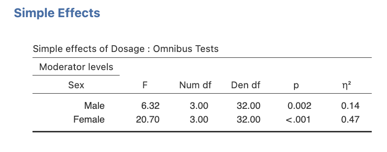
(This output does not have the partial eta squared or beta, but if you left those boxes ticked in Step 2.6, you will see them too.)
- Figure out where the output displays the cell and marginal means (in the ‘Descriptive Statistics’ section). Note that the marginal means will be the ‘total’ means for each variable level.
- Determine in which output table the simple effects test results are displayed.
Task 1: Take a look at the output above and write the key bits of information into the summary table below (as we did for the omnibus tests in Activity 2: Exercise 4).
Download Table 3.4 (PDF, 133 KB) to write the information.
Table 3.4
Summary Table for Simple Effects
|
Source |
|
SS |
df |
MS |
F |
p |
|
Effect of Dosage at S1 |
||||||
|
Effect of Dosage at S2 |
||||||
|
(Corrected) Total |
|
|
|
|
|
|
Go to a version of Table 3.4 formatted for accessibility.
If exact p-values were not provided, you could compare your F obtained for each simple effect to the F critical value in F tables (with the appropriate df). This critical value would be:
Fα = .05(3, 32) = 2.86
Double-check that your decision regarding significance/ non-significance for each of the above simple effects remains the same using this other criterion.
Task 2:
*** You have not yet completely finished with the simple effects of drug dosage. More follow-up is needed, because we don’t yet know where the differences in dosage are for males or females (i.e., we will need to do simple comparisons). This will be covered next in Exercise 8. ***
Exercise 8: Follow-up Tests for an Interaction – Simple Comparisons
Given that the simple effects of drug dosage were significant (note that they were significant both for males and females), we need to go one step further to locate where the differences in maze running performance at the different dosage levels lie. Therefore, this time we will be comparing CELL means. As we are performing the comparisons to follow up significant simple effects (which in themselves were conducted to follow up a significant interaction), we call these ‘simple comparisons’.
Remember, our third hypothesis was:
“The effect of drug dosage will differ for males compared to females. While both sexes will exhibit increased performance when they receive any amount of the drug than when they do not, the particular benefits of the small drug dosage (compared to the large dose) will be more noticeable in female rats than in male rats.”
So again, our hypothesis lends itself to investigation via pairwise comparisons in jamovi!
Task 1
The answer is that there are eight pairwise comparisons needed to address Hypothesis 3, which mirror that for the main effect follow-up tests. Namely, for male and for female rats we want to examine:
- zero vs. small drug dosage,
- zero vs. moderate drug dosage,
- zero vs. large drug dosage, and
- small vs. large drug dosage.
These four will be performed once for males and again for females, providing eight simple comparisons in total. However, since we will be conducting four comparisons to follow up each significant simple effect (i.e., the simple effect of dosage for males, and the simple effect of dosage for females), this means that each set contains only four follow-up tests. Hence when we are assessing whether or not to employ a Bonferroni correction to our αcritical level, we will use this number of comparisons in each set to help form our decision (i.e., four). In our case, since we plan to conduct four pairwise t-tests to follow up each of our significant simple effects, which are specifically designed to test our Hypothesis 3 predictions within a small data set in an established research area, then an adjustment should NOT be applied to αcritical for the number of tests performed (i.e., no Bonferroni correction; see Conservative Follow-Up Tests for Main Effect Comparisons as a guide to when an αcritical adjustment is appropriate).
As stated above, since Hypothesis 3 is worded in such a way that pairwise simple comparisons can be performed (i.e., comparing only two groups at a time rather than multiple groups), we can run simple comparison results in the jamovi via the ANOVA menu results we have run before. Remember however, at the end of the day, you have a choice to adopt either a linear contrast or pairwise approach to your main and/ or simple comparisons. This choice should be driven by your research questions and underlying theory!
Recall that we will ask for pairwise simple comparisons with no correction to αcritical (i.e., it employs the LSD adjustment method). Therefore, if we had want to apply a Bonferroni correction we will have to do so by hand, just as we would for main comparisons. Consequently, the procedure for this is exactly the same as that taught earlier in Exercise 6 for the hypothetical example, except this time the method would be applied to simple comparisons. Hence, we would find the relevant p-values to compare to our new Bonferroni adjusted αcritical in a different output table i.e., the Pairwise Comparisons table.
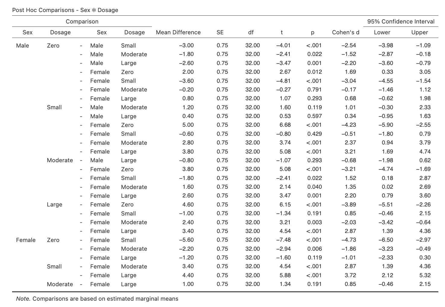
Step 1: Obtain the Simple Comparisons That Accompany These Simple Effects.
The best way to obtain these is to scroll up in your jamovi and go back to the original ANOVA in your results output (the one produced in Exercise 5 Step 2). Go to the Post Hoc Tests drop down list and this time select the interaction term (Sex*Dosage) and move it across to the right hand side box. Ensure that No correction is selected under the Correction heading.
The relevant output you will obtain from this is shown below.
Figure 3.7
Simple Comparisons for the Dosage Simple Effects for Male and Female Rats
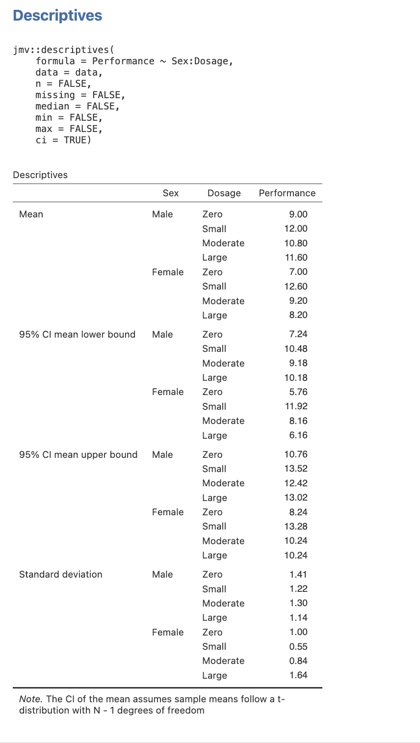
Step 2: Getting Our Cell Means and Standard Deviations in jamovi
- Select the Analyses menu.
- Click Exploration, then Descriptives.
- Select the dependent variable (i.e., Performance) and then click on the arrow button to move the DV into the Variables box.
- Select the independent variables in turn (i.e., Sex and Dosage) and click on the arrow button to move each variable into the Split by box.
- In the Statistics drop down menu ensure that you have the Mean checkbox under the Central Tendency section ticked, and the Std. deviation checkbox under the Dispersion section ticked. Finally, check the Confidence interval for Mean checkbox under Mean Dispersion. You can unselect all other default selections to get a table that has only the means and standard deviations you need.
Here is the table you will get when you follow this process.
Figure 3.8
Descriptive Statistics for the Simple Comparisons
Task 2
Referring to the jamovi output containing the pairwise simple comparisons, determine which of our key simple comparisons are significant. Write your answers in the space provided.
State the significance/ non-significance and direction of each of the eight relevant simple comparisons.
Task 3
Write up the results for the simple comparisons of drug dosage for both males and females.
State in words what the results mean. That is, explain first that simple comparisons were performed via a series of pairwise t-tests in order to follow up the significant simple effect of drug dosage for males/ females. Report the number of comparisons conducted, and the α-level used for each comparison. If a correction to α critical was employed, state what type (NB: if no adjustment was performed, this last piece of information is typically omitted). Then, for each comparison, state the significance and report the direction of effect (complete with the relevant statistical notation, and cell means and standard deviations). Be sure to group all the follow-up tests for males together, and then report all the follow-up tests for the females, as this makes for a more logical and easy-to-follow presentation of results.
Task 4: The Full Write Up
Now you can piece together the write up from Exercise 4 in Activity 2 with the write ups you have just done. That is, you can report (in the following order):
- The overall type of analysis that was performed, stating what the IV(s) and DV were. This includes specifying the levels of the IV(s). Again, recall that by convention, we tend to use specific notation to present this information in a condensed manner.
- The main effect of sex – remember to state significance and the direction of effect.
- The main effect of drug dosage, stating its significance.
- Then, report the main effect comparisons (stating the significance and direction of effect for each).
- The interaction – state its significance.
- The simple effects of drug dosage – state the significance of each (i.e., for both males and females).
- Report the simple comparisons of drug dosage, for males and then for females. Be sure to group these following their relevant simple effect that they are following up. I.e., the simple comparisons of dosage for males should be reported immediately after the significant simple effect of dosage for males, while the simple comparisons of dosage for females should be reported immediately following the significant simple effect of dosage for females.
Don’t forget to include relevant:
- Statistical notation after each of the omnibus and simple effects tests (i.e., F, df, p, η2 or ω2). Remember that all the omnibus and simple effects tests will need an effect size!
- Statistical notation after each main/ simple comparison (i.e., t, df, p, d, and 95% CI).
- Marginal/ cell means and standard deviations when describing the direction of effect. NB: These statistics are only reported once each and not repeated i.e., they are given the first time the relevant group is mentioned in the text.
- Information about the type of main/ simple comparisons that were performed, including:
a) Whether they were pairwise t-tests or linear contrasts,
b) The number of comparisons conducted,
c) The critical α-level employed for each comparison, and
d) What type of correction to αcritical was used (NB: if no adjustment was performed, this last piece of information is typically omitted).
As a reminder:
- Statistical notation in English/ Latin letters needs to be italicised (e.g., F, t, p, d), while that in Greek (e.g., η2, ω2) appears as standard text. Likewise, notation for subscripts and superscripts are presented in standard text (i.e., these do not appear in italics).
- Inferential statistics (e.g., F, t), effect sizes (e.g., η2, ω2, d) should be presented to two decimal places, while p-values go to three.
- Descriptive statistics are given to the number of decimals commensurate with their precision of measurement. In our case, means and standard deviations should be taken to one decimal place for reporting.
- Values that can potentially exceed a threshold of ±1 (e.g., M, SD, F, t, d), should have a 0 preceding the decimal point. However, values that cannot potentially exceed ±1 (e.g., p, η2, ω2), should not have a 0 before the decimal.
- The direction of effect for main/ simple comparisons should also be reflected in the positive or negative valence of the reported t-value. That is, a positive t-value indicates the first reported group involved in the comparison had a higher mean than the second group. In contrast, a negative t-value indicates that the first reported group involved in the comparison had a lower mean than the second group.
With all this information, you have a complete write-up for a 4 x 2 between groups factorial ANOVA!
Note. It is common to provide a figure that accompanies a write up such as this, in order to illustrate the significant interaction. Recall that this should have the DV on the y-axis [i.e., Maze Running Performance (1-15)], the key factor on the x-axis (i.e., drug dosage) and the proposed moderator as separate lines on the graph (i.e., sex). The points presented on the graph will be the dosage x sex cell means. Don’t forget that this will also require error bars.
Alternative Multiple Comparison Procedures
In the hypothetical example provided in Exercise 6 earlier, we followed up our significant main effect with more than two levels using main comparisons with a Bonferroni correction to αcritical for five pairwise t-tests (αFW = .05). This adjusted the critical significance value based on the number of tests that were performed, where each of the five comparisons was conducted at α = .01. Having said this, any post hoc comparison technique could also be used to follow up significant main or simple effects with more than two levels when a more conservative approach is required [e.g., Tukey’s, Scheffé’s; see Howell (2010) Chapter 12 sections 12.6 and especially 12.7, pp. 389-398]. These procedures all adjust the critical α value against which we evaluate our calculated t-test statistic, so as to maintain familywise error rate at α = .05 (or α = .01).
Full Copy of the JAMOVI Output From Between Groups Factorial ANOVA Section
Now that you have completed the full analysis for the between groups factorial ANOVA, here is a copy of the JAMOVI file that contains the full set of analysis output that we have conducted. You can cross check this with the analysis you have conducted to check you have conducted it correctly.
Download the Factorial BG ANOVA final analysis output and data (omv, 21 KB)
Test Your Understanding
- Explain the difference between a priori and post hoc tests in doing main or simple comparisons. Which is preferred, and why?
- Why is it important to control familywise error rate when performing (a) five or more main/ simple effect comparisons, or (b) when performing post hoc (rather than a priori planned) comparisons? Explain, using an example.
- A researcher is interested in testing the efficacy of cognitive-behavioural therapy on children’s attachment problems. They want to test their own theory that the efficacy of this particular treatment in improving healthy attachment is related to the degree of parental involvement in the therapy. To test this, the researcher randomly allocates 60 children to either a cognitive-behavioural or control therapy group. From here, they further randomly assign children to one of three conditions. A third of the children in each therapy group participate in one-on-one treatment with the researcher (control condition), a third have one parent present (condition 1), and the remaining third have both parents present (condition 2). Outline the results you might anticipate, given the researcher’s hypotheses. What a priori tests of simple effects would you set up, if any?
