
Solutions
[latex]\newcommand{\pr}[1]{P(#1)} \newcommand{\var}[1]{\mbox{var}(#1)} \newcommand{\mean}[1]{\mbox{E}(#1)} \newcommand{\sd}[1]{\mbox{sd}(#1)} \newcommand{\Binomial}[3]{#1 \sim \mbox{Binomial}(#2,#3)} \newcommand{\Student}[2]{#1 \sim \mbox{Student}(#2)} \newcommand{\Normal}[3]{#1 \sim \mbox{Normal}(#2,#3)} \newcommand{\Poisson}[2]{#1 \sim \mbox{Poisson}(#2)} \newcommand{\se}[1]{\mbox{se}(#1)} \newcommand{\prbig}[1]{P\left(#1\right)}[/latex]
1. Variability
| Sex | Nominal |
| Age | Discrete |
| Height | Continuous |
| Weight | Continuous |
| Forearm | Continuous |
| Pulse | Discrete (by the way it was obtained) |
| Eyes | Nominal |
| Pizza | Nominal |
| Education | Ordinal |
| Kiss | Nominal |
2. Designing Studies
Exercise 1
Suppose the groups are A, B and C. There are many ways we could assign the 20 subjects randomly to these groups using Table 2.2. For example, suppose we want to have roughly equal groups, so perhaps 7 in A and B and 6 in C. Assign the digits 0-2 to A, 3-5 to B and 6-8 to C (and if 9 comes up we ignore it).
The first digit is 8 so we assign the first subject to C. The second digit is 7 so we assign the second to C, as we then also do with the third. The fourth digit is 2 and so we assign the fourth subject to A. Continuing on in this way we obtain the allocation:
| Group | Subject | ||||||
| A | 4 | 8 | 15 | 16 | 18 | 19 | 20 |
| B | 6 | 7 | 10 | 11 | 13 | 14 | 17 |
| C | 1 | 2 | 3 | 5 | 9 | 12 | |
Exercise 2
The largest difference in means would occur if the 10 highest increases were allocated to the caffeine group, as in the following table:
| Caffeine | 10 | 12 | 15 | 16 | 16 | 17 | 20 | 21 | 22 | 27 |
| Caffeine-free | -9 | -2 | 4 | 4 | 5 | 5 | 6 | 6 | 7 | 7 |
This gives a mean increase of 17.6 bpm for the caffeine group and 3.3 bpm for the caffeine-free group, a difference of 14.3 bpm.
Exercise 3
- Let [latex]\mu_M[/latex] and [latex]\mu_F[/latex] be the mean weight of males and females, respectively, around this height. Alice is interested in testing
\[ H_0: \mu_M = \mu_F \mbox{ versus } H_1: \mu_M > \mu_F. \] - The observed means are
\[ \overline{x}_M = \frac{226}{3} = 75.33, \]
\[ \overline{x}_F = \frac{215}{4} = 53.75, \]
giving a mean difference of [latex]\overline{x}_M - \overline{x}_F = 21.58[/latex] kg. - If [latex]H_0[/latex] is true then there is no difference between males and females. The [latex]P[/latex]-value is the probability of obtaining a difference as large as 21.58 simply by randomly allocating the male and female labels to the 7 observations. There are only
\[ {7 \choose 4} = {7 \choose 3} = 35 \]
ways of doing this allocation so we could calculate the exact [latex]P[/latex]-value by working out the mean difference for each of these and seeing whether it is as large as 21.58 kg.Alternatively, we can look at the data and think about how many ways we could obtain a larger difference. In fact there is only one: if the 68 was female and the 70 was male we would obtain a larger mean difference, and no other allocation would give a larger difference. Thus, of the 35 possibilities, there are 2 ways of obtaining a difference as large as 21.58, the one we observed and this other one. The probability of obtaining a difference as large as 21.58 by chance is then
\[ \frac{2}{35} = 0.057. \]
This is fairly inconclusive evidence of a difference in mean weights.
Exercise 4
As with the previous exercise, we want to know how many of the
\[ {10 \choose 5} = 252 \]
allocations of values to groups would give a mean difference as large as the one observed. The following table shows the original data but here we have put the values in order and indicated group membership below each value.
| 1045 | 1051 | 1182 | 1366 | 1444 | 1460 | 1568 | 1629 | 1739 | 1822 |
| D | D | D | R | D | R | R | D | R | R |
The sum of the values labelled R is 7955. Note that we will obtain a larger difference if sum in the Rested group is larger than this sum (since the total of all the values is fixed). The sum will be larger if some of the R labels were placed on higher values. We can extend the table by systematically working through all the ways of doing this:
| 1045 | 1051 | 1182 | 1366 | 1444 | 1460 | 1568 | 1629 | 1739 | 1822 | Sum |
| D | D | D | R | D | R | R | D | R | R | 7955 |
| D | D | D | D | R | R | R | D | R | R | 8033 |
| D | D | D | R | D | R | D | R | R | R | 8016 |
| D | D | D | D | R | R | D | R | R | R | 8094 |
| D | D | D | R | D | D | R | R | R | R | 8124 |
| D | D | D | D | R | D | R | R | R | R | 8202 |
| D | D | D | D | D | R | R | R | R | R | 8218 |
| D | D | D | R | R | D | D | R | R | R | 8000 |
So we have found 8 possible ways of obtaining a sum of 7955 or larger in the Rested group. If the group labels were allocated at random then the probability of obtaining a difference as large as observed is
\[ \frac{8}{252} = 0.032. \]
Although both groups seem to overestimate the duration, this [latex]P[/latex]-value gives some evidence that the sleep-deprived subjects tend to give a lower estimate than the rested subjects.
3. Visualising Distributions
Exercise 1
The histogram below shows a distribution of breath holding times that seems to be bimodal:

A side-by-side dot plot shows clearly that this bimodal distribution arises from sex difference in breath holding times:

Exercise 2
Based on a lattice plot showing separate histograms for the two groups, it appears there is little difference in the two distributions.

A side-by-side dot plot suggests a similar conclusion and also shows clearly the plants that died in each group:

Exercise 3
There are 15 with purple eyes, 16 with green, 5 with brown and 14 with blue, giving a total of 50 in the sample. The proportion with blue eyes is thus
\[ \frac{14}{50} = 0.28. \]
4. Quantiles
Exercise 1
The 60 age observations in order are
| 15 | 15 | 16 | 16 | 17 | 18 | 19 | 19 | 19 | 19 | 19 | 20 | 20 | 21 | 22 |
| 22 | 23 | 23 | 23 | 23 | 23 | 24 | 25 | 25 | 27 | 27 | 28 | 29 | 30 | 33 |
| 33 | 35 | 35 | 36 | 36 | 36 | 36 | 37 | 37 | 38 | 39 | 39 | 40 | 41 | 41 |
| 42 | 43 | 43 | 45 | 45 | 47 | 48 | 52 | 54 | 56 | 57 | 58 | 58 | 60 | 61 |
With an even number of observations, the median will be the average of the two numbers on each side of the median position. The 30th value is 33 years while the 31st value is also 33 years, making the median age 33 years.
Exercise 2
To find the median we first need to know how many forearm observations were collected. The figure shows the count for each reported length (assuming that values were given to the nearest centimetre). Adding all these counts together gives
\[ 1+1+4+3+3+2+2+5+5+11+9+3+1 = 50. \]
Thus the median is the average of the 25th and 26th forearm observations when placed in order. Looking at the counts, observations 22-26 are all 24 cm. Thus the median forearm length is 24 cm.
Exercise 3
The 60 weight observations in order are
| 45 | 46 | 48 | 52 | 53 | 53 | 54 | 54 | 54 | 55 | 57 | 57 | 57 | 57 | 58 |
| 59 | 59 | 59 | 59 | 60 | 60 | 60 | 61 | 62 | 62 | 62 | 63 | 64 | 64 | 65 |
| 65 | 66 | 67 | 67 | 68 | 68 | 68 | 69 | 71 | 71 | 72 | 72 | 72 | 74 | 74 |
| 75 | 76 | 76 | 77 | 79 | 79 | 79 | 80 | 81 | 81 | 85 | 85 | 95 | 100 | 109 |
With an even number of observations, the median position is between the 30th and 31st values. Thus we can take the first quartile to be the median of the first 30 observations. Since this is an even number, the median of these is the average of the 15th and 16th values, [latex]Q_1 = 58.5[/latex] kg.
Similarly, the third quartile will be the average of the 45th and 46th values, [latex]Q_3 = 74.5[/latex] kg.
Exercise 4
Side-by-side dot plots and box plots show no substantial differences between the male and female distributions for reaction times:


A quantile-quantile plot could also be used here to show that the two distributions match quite closely:

Exercise 5
The side-by-side box plots again show little difference between the two groups:

Note however that the box plots are not such good pictures of the distributions since they don’t show the plants that died as clearly as the dot plots and histograms in Exercise 3.2.
5. Averages
Exercise 1
If the mean height of 8 people is 172 cm then their total combined height is
\[ 8 \times 172 = 1376 \mbox{ cm}. \]
If the mean height of the 7 people remaining is 171 cm then their total combined height is
\[ 7 \times 171 = 1197 \mbox{ cm}. \]
Thus the height of the person who left must be
\[ 1376 – 1197 = 179 \mbox{ cm}.\]
Exercise 2
The mean height of the 26 females in the survey was 167.4 cm. The following table shows the squared deviations from this mean for the 26 heights:
| [latex](174-167.4)^2[/latex] | 43.56 |
| [latex](160-167.4)^2[/latex] | 54.76 |
| [latex](169-167.4)^2[/latex] | 2.56 |
| [latex](174-167.4)^2[/latex] | 43.56 |
| [latex](166-167.4)^2[/latex] | 1.96 |
| [latex](166-167.4)^2[/latex] | 1.96 |
| [latex](166-167.4)^2[/latex] | 1.96 |
| [latex](171-167.4)^2[/latex] | 12.96 |
| [latex](166-167.4)^2[/latex] | 1.96 |
| [latex](164-167.4)^2[/latex] | 11.56 |
| [latex](169-167.4)^2[/latex] | 2.56 |
| [latex](165-167.4)^2[/latex] | 5.76 |
| [latex](177-167.4)^2[/latex] | 92.16 |
| [latex](170-167.4)^2[/latex] | 6.76 |
| [latex](178-167.4)^2[/latex] | 112.36 |
| [latex](173-167.4)^2[/latex] | 31.36 |
| [latex](175-167.4)^2[/latex] | 57.76 |
| [latex](155-167.4)^2[/latex] | 153.76 |
| [latex](171-167.4)^2[/latex] | 12.96 |
| [latex](156-167.4)^2[/latex] | 129.96 |
| [latex](165-167.4)^2[/latex] | 5.76 |
| [latex](165-167.4)^2[/latex] | 5.76 |
| [latex](165-167.4)^2[/latex] | 5.76 |
| [latex](167-167.4)^2[/latex] | 0.16 |
| [latex](159-167.4)^2[/latex] | 70.56 |
| [latex](167-167.4)^2[/latex] | 0.16 |
| Total | 870.36 |
The variance for female heights is thus
\[ \frac{870.36}{26-1} = 34.81 \mbox{ cm}^2, \]
giving a standard deviation of [latex]\sqrt{34.81} = 5.90[/latex] cm. The calculation is similar for the 34 male heights.
Exercise 3
The mean number of leaves for the control group is
\[ \frac{8 + 6 + 6 + 4 + 5 + 6}{6} = \frac{35}{6} = 5.83 \mbox{ leaves} \]
while for the fertilizer group the mean is
\[ \frac{11 + 8 + 9 + 8 + 8 + 0}{6} = \frac{44}{6} = 7.33 \mbox{ leaves}. \]
It seems the fertilizer group has done a bit better on average. However, if we ignored the plant that died the fertilizer mean would change to
\[ \frac{11 + 8 + 9 + 8 + 8}{5} = \frac{44}{5} = 8.80 \mbox{ leaves}. \]
This is a better result but at the price of discarding a plant where the fertilizer may have been harmful. It is thus a scientific question as to whether or not we should include this value, based on whether or not the fertilizer may have been related to the fungal infection.
In contrast the median number of leaves for the control group is 6 while for the fertilizer group it is 8. This median doesn’t change if we ignore the plant that died.
The corresponding standard deviations are
\[ \sqrt{\frac{8.33}{6-1}} = 1.33 \mbox{ leaves} \]
for the control group and
\[ \sqrt{\frac{71.33}{6-1}} = 3.78 \mbox{ leaves} \]
for the fertilizer group. The value for the fertilizer group is greatly inflated by the 0 value. Ignoring that value reduces the standard deviation to
\[ \sqrt{\frac{6.80}{5-1}} = 1.30 \mbox{ leaves}, \]
very similar to the control group value.
Finally, the quartiles are [latex]Q_1 = 5[/latex] and [latex]Q_3 = 6[/latex] for the control group and [latex]Q_1 = 8[/latex] and [latex]Q_3 = 9[/latex] for the fertilizer group, giving interquartile ranges of 1 leaf for both groups. With such small numbers of observations the interquartile range can be very sensitive. Here removing the 0 value leaves [latex]Q_1 = 8[/latex] but increases [latex]Q_3[/latex] to [latex]\frac{9+11}{2} = 10[/latex].
Exercise 4
Let [latex]f(b)[/latex] be the sum of the squared prediction errors for a particular estimate, [latex]b[/latex], so that
\[ f(b) = \sum_{j=1}^n (x_j – b)^2, \]
as given on page 63. To find the minimum value of this sum we want to find where its first derivative is equal to 0. Here
\[ f'(b) = \sum_{j=1}^n -2(x_j – b) = \left( -2 \sum_{j=1}^n x_j \right) + \left( 2 \sum_{j=1}^n b \right). \]
We have separated the sum into its two components. Note that in the second sum we are just adding up [latex]b[/latex] a total of [latex]n[/latex] times, so this is just [latex]n b[/latex]. Thus we want
\[ \left(-2 \sum_{j=1}^n x_j\right) + 2 n b = 0 \Rightarrow n b = \sum_{j=1}^n x_j, \]
so we have a minimum when
\[ b = \frac{\sum_{j=1}^n x_j}{n}. \]
This is just the sample mean of the [latex]x_j[/latex] values, as required.
6. Visualizing Relationships
Exercise 1
The figure below shows a scatter plot of height against forearm with the unusual forearm value corrected. A \emph{loess} curve has been added (in lieu of drawing one by hand).

Overall the relationship is positive and fairly linear, though it is influenced by the large forearm value. The relationship seems moderately strong.
Exercise 2
The counts are given in the following table:
| Mushroom | Pineapple | Prawns | Sausage | Spinach | Total | |
| Female | 22 | 33 | 17 | 14 | 18 | 104 |
| Male | 21 | 8 | 11 | 30 | 26 | 96 |
| Total | 43 | 41 | 28 | 44 | 44 | 200 |
Dividing each row through by its row total will give the pizza preference proportions conditional on sex:
| Mushroom | Pineapple | Prawns | Sausage | Spinach | Total | |
| Female | .212 | .317 | .163 | .135 | .173 | 1.000 |
| Male | .219 | .083 | .115 | .312 | .271 | 1.000 |
A segmented bar chart of these conditional proportions is given below:

It appears there may be sex differences in pizza preference in Providence.
Exercise 3
A time plot is given below with the old and new wires shown separately.

It appears the estimates using the old wire may have been slightly lower than with the new wire.
Exercise 4
The bar chart below shows the distribution of education level conditional on sex.

7. Linear Relationships
Exercise 1
From the scatter plot below there seems to be a strong non-linear negative relationship between dissolving time and volume.

This does not seem to be an exponential relationship since there is a vertical asymptote — plotting [latex]\log_{10}(\mbox{Time})[/latex] against Volume doesn’t make the pattern linear. Instead the relationship appears more like a hyperbola, or more generally a power relationship
\[ y = a x^b. \]
Taking logarithms of both sides gives
\[ \log_{10}(y) = \log_{10}(a x^b) = \log_{10}(a) + \log_{10}(x^b) = \log_{10}(a) + b \log_{10}(x). \]
This now has the form of a linear relationship between [latex]\log_{10}(y)[/latex] and [latex]\log_{10}(x)[/latex] where the intercept is [latex]\log_{10}(a)[/latex] and the slope is [latex]b[/latex]. The figure below shows the scatter plot of [latex]\log_{10}(\mbox{Time})[/latex] against [latex]\log_{10}(\mbox{Volume})[/latex] with the fitted least-squares line:

The fit seems quite good, with [latex]\log_{10}(a) = 1.4481[/latex] and [latex]b = -0.5864[/latex]. Reversing the transformation then gives
\[ \mbox{Time} = 10^{1.4481} \times \mbox{Volume}^{-0.5864} = 28.06 \times \mbox{Volume}^{-0.5864}. \]
The final figure shows the original scatter plot with this curve added:

Exercise 2
On the Forearm axis the scale is roughly 6 mm on paper for each centimetre of forearm length. You can use this and a ruler to estimate the forearm length from the line for a height of 160 cm to be 24.2 cm. Similarly for a height of 180 cm we estimate the estimate to be 25.8 cm. This gives an increase in forearm length for 20 cm of height to be
\[ 25.8 – 24.2 = 1.6 \mbox{ cm}. \]
Thus the estimated forearm length for a height of 100 cm would be
\[ 24.2 – 3 \times 1.6 = 19.4 \mbox{ cm}. \]
Note that this is just an exercise in reading a plot and working with lines and slopes. In practice it would not make sense to estimate a value so far out of the range of the data.
Exercise 3
For [latex]x = 3[/latex] we have
\[ \log_{10} y = 0.810 + 2.669 \log_{10} 3 = 0.810 + 2.669 \times 0.4771 = 2.083, \]
giving an estimated response ([latex]y[/latex]) value of
\[ y = 10^{2.083} = 121.2. \]
Exercise 4
The following scatterplot shows a relationship with a correlation of exactly 0. The line shown is the fitted least squares regression line, correspondingly with 0 slope.

Exercise 5
The mean [latex]x[/latex] value is
\[ \overline{x} = \frac{x_1 + x_2}{2}, \]
giving variance
\begin{eqnarray*}
s_x^2 & = & \frac{\left(x_1 – \frac{x_1 + x_2}{2}\right)^2 + \left(x_2 – \frac{x_1 + x_2}{2}\right)^2}{2-1} \\
& = & \left( \frac{x_1 – x_2}{2} \right)^2 + \left( \frac{x_2 – x_1}{2} \right)^2 \\
& = & \frac{(x_1 – x_2)^2}{2}, \\
\end{eqnarray*}
so that the standard deviation is
\[ s_x = \frac{|x_1 – x_2|}{\sqrt{2}}, \]
with corresponding values for [latex]y[/latex].
Proceeding to the correlation coefficient, we have terms such as
\[ \frac{x_1 – \overline{x}}{s_x} = \frac{1}{\sqrt{2}} \frac{x_1 – x_2}{|x_1 – x_2|}. \]
If [latex]x_1 > x_2[/latex] then this is [latex]\frac{1}{\sqrt{2}}[/latex] while if [latex]x_1 x_2[/latex] it is [latex]-\frac{1}{\sqrt{2}}[/latex]. Supposing [latex]x_1 > x_2[/latex] and [latex]y_1 > y_2[/latex], the value of
\[ \left( \frac{x_1 – \overline{x}}{s_x} \right) \left( \frac{y_1 – \overline{y}}{s_y} \right) + \left( \frac{x_2 – \overline{x}}{s_x} \right) \left( \frac{y_2 – \overline{y}}{s_y} \right) \]
will be
\[ \left( \frac{1}{\sqrt{2}} \right) \left( \frac{1}{\sqrt{2}} \right) + \left( -\frac{1}{\sqrt{2}} \right) \left( -\frac{1}{\sqrt{2}} \right) = 1, \]
whereas if [latex]x_1 > x_2[/latex] but [latex]y_1 y_2[/latex], the value is
\[ \left( \frac{1}{\sqrt{2}} \right) \left( -\frac{1}{\sqrt{2}} \right) + \left( -\frac{1}{\sqrt{2}} \right) \left( \frac{1}{\sqrt{2}} \right) = -1. \]
This is not surprising since with two points we will always have a perfect positive or negative linear relationship. Note that we could only get a value of 0 above if, for example, [latex]x_1 = x_2[/latex]. However, this would give [latex]s_x = 0[/latex] and so the correlation would be undefined.
8. Probability
Exercise 2
The odds of the event are
\[ 1.78 = \frac{p}{1 - p}, \]
where [latex]p[/latex] is the probability of that event. We can rearrange this to give
\[ 1.78 - 1.78p = p, \]
so that
\[ p = \frac{1.78}{1 + 1.78} = 0.6403. \]
In general, if the odds are [latex]q[/latex] then
\[ p = \frac{q}{1 + q}. \]
Exercise 3
Calculating the log-odds uses natural logarithms so if the log-odds were -1.266 then the odds are
\[ e^{-1.266} = \exp(-1.266) = 0.2820. \]
We can then use the formula from the previous exercise to find
\[ p = \frac{0.2820}{1 + 0.2820} = 0.2200. \]
Exercise 4
The surprisal is
\[ 2.5 = -\log_2(p), \]
so that
\[ p = 2^{-2.5} = 0.1768. \]
A surprisal of 2.5 is between getting all heads from 2 coins tosses and getting all heads from 3 coin tosses. These probabilities are 0.25 and 0.125, respectively, so the value we have found makes sense.
Exercise 5
The probability is the area of the rectangle so that for a particular height, [latex]x[/latex], we have
\[ p = P(X \ge x) = (190 - x) \times h = (190 - x) \times \frac{1}{40}. \]
Rearranging this gives
\[ x = 190 - 40p. \]
For example, the third quartile of this distribution, where [latex]p = 0.25[/latex], is
\[ x = 190 - 40 \times 0.25 = 180 \mbox{ cm}, \]
as expected from the figure.
Exercise 6
The triangular density in makes this question a lot more messy than the previous exercise. It will be useful to consider the two halves of the triangle separately. For [latex]x \ge 170[/latex] the right tail is a triangle with
\[ p = P(X \ge x) = \frac{1}{2}(190 - x) \left( \frac{190 - x}{20} \right) \frac{1}{20}. \]
Here [latex]\frac{190 - x}{20}[/latex] is the proportion of the overall height, [latex]\frac{1}{20}[/latex], obtained for a particular value of [latex]x[/latex], with the maximum at [latex]x = 170[/latex]. This expression simplifies to
\[ p = \frac{(190-x)^2}{800}, \]
so we have
\[ x = 190 - 20\sqrt{2p}. \]
From this expression the third quartile is where
\[ x = 190 - 20\sqrt{2 \times 0.25} = 190 - 20 \times 0.7071 = 175.9 \mbox{ cm}. \]
For [latex]x \lt 170[/latex] we can write the area to the right as
\[ p = P(X \ge x) = 1 - \frac{1}{2}(x - 150) \left( \frac{x - 150}{20} \right) \frac{1}{20}. \]
Here we are working out the area to the left and subtracting this value from 1 to obtain the area [latex]P(X \ge x)[/latex]. This expression for [latex]p[/latex] simplifies to
\[ p = 1 - \frac{(x - 150)^2}{800}, \]
so now
\[ x = 150 + \sqrt{800 - 800p} = 150 + 20\sqrt{2(1-p)}. \]
For example, the first quartile is where
\[ x = 150 + 20\sqrt{2 \times (1-0.75)} = 150 + 20 \times 0.7071 = 164.1 \mbox{ cm}. \]
Exercise 7
Since the total area must be 1 we have
\[ \frac{1}{2}(100 - 40)h = 1 \]
so [latex]h = \frac{1}{30}[/latex]. Now 50 kg is half way between 40 kg and 60 kg so the height of the line at 50 kg is half way between 0 and [latex]h[/latex], a value of [latex]\frac{1}{60}[/latex]. Thus the area of the triangle below 50 kg is
\[ \frac{1}{2}(50 - 40)\frac{1}{60} = \frac{1}{12}, \]
so the probability of being less than 50 kg is [latex]\frac{1}{12}[/latex].
More generally, for a weight [latex]x[/latex] between 60 and 100, the height of the line is
\[ \frac{100 - x}{100 - 60} h = \frac{100 - x}{1200}. \]
We thus want to solve
\[ \mbox{Area } = \frac{1}{2} (100 - x) \frac{100 - x}{1200} = \frac{(100 - x)^2}{2400} = 0.1. \]
Rearranging gives
\[ 100 - x = \sqrt{240}, \]
so [latex]x = 100 - \sqrt{240} = 84.5[/latex] kg is the weight needed to be in the top 10% of weights.
9. Conditional Probability
Exercise 1
Suppose [latex]p[/latex] is the true proportion of students who have cheated on an exam. There are two ways a students could respond yes to the question, through being told to answer honestly or through being told to answer yes by the die. The total probability is
\[ \pr{\mbox{Yes}} = \pr{\mbox{1 or 2}} \pr{\mbox{Yes } | \mbox{ 1 or 2}} + \pr{\mbox{3 or 4}} \pr{\mbox{Yes } | \mbox{ 3 or 4}}. \]
Now both of [latex]\pr{\mbox{1 or 2}} = \pr{\mbox{3 or 4}} = \frac{1}{3}[/latex]. If they answer honestly then the probability they will say Yes is [latex]p[/latex], so
\[ \pr{\mbox{Yes } | \mbox{ 1 or 2}} = p. \]
If it comes up 3 or 4 then they always say yes, so
\[ \pr{\mbox{Yes } | \mbox{ 3 or 4}} = 1. \]
Thus
\[ \pr{\mbox{Yes}} = \frac{1}{3} \times p + \frac{1}{3} \times 1 = \frac{p + 1}{3}. \]
We can estimate this probability using the sample proportion of students answering yes, [latex]\frac{33}{60} = 0.55[/latex]. That is,
\[ \frac{p + 1}{3} \approx 0.55 \Rightarrow p \approx 3 \times 0.55 - 1 = 0.65. \]
Thus we estimate that the true proportion of students who have cheated on an exam is about 65%.
Exercise 2
Consider the suggestion of using a deck of cards to establish anonymity. With a regular deck we could use red cards to indicate that they should answer truthfully and black cards to always answer yes. Following the structure from the previous exercise, we have
\[ \pr{\mbox{Yes}} = \pr{\mbox{Red}} \pr{\mbox{Yes } | \mbox{ Red}} + \pr{\mbox{Black}} \pr{\mbox{Yes } | \mbox{ Black}}. \]
Suppose [latex]p[/latex] is the true proportion of respondents who would say yes to the question of interest. Then
\[ \pr{\mbox{Yes}} = \frac{1}{2} \times p + \frac{1}{2} \times 1 = \frac{p + 1}{2}. \]
While this is a simple method to use it is of course the case that anyone who says no must be truthfully saying no. This may not be such an issue if only a yes response was considered sensitive.
Exercise 3
The probability that someone tests positive for cervical cancer is made up of two groups, the people with cervical cancer and those without cervical cancer. That is,
\begin{align*}
\pr{\mbox{Positive}} & = \pr{\mbox{Cancer}} \pr{\mbox{Positive } | \mbox{ Cancer}} \\
& + \pr{\mbox{No Cancer}} \pr{\mbox{Positive } | \mbox{ No Cancer}}.
\end{align*}
From the information given we have
\[ \pr{\mbox{Cancer}} \pr{\mbox{Positive } | \mbox{ Cancer}} = 0.086 \times 0.927 = 0.07972. \]
That is, 7.972% of the population group will have cervical cancer \emph{and} will test positive.
Based on the specificity, the probability of a positive result for someone without cervical cancer is [latex]1 - 0.854 = 0.146[/latex]. The proportion of the population without the cancer is [latex]1 - 0.086 = 0.914[/latex], so we have
\[ \pr{\mbox{No Cancer}} \pr{\mbox{Positive } | \mbox{ No Cancer}} = 0.914 \times 0.146 = 0.13344. \]
So 13.344% of the population group will not have cervical cancer \emph{and} will test positive.
The total proportion who would test positive is thus
\[ 0.07972 + 0.13344 = 0.21316. \]
The proportion of this total who actually have the cancer is
\[ \frac{0.07972}{0.21316} = 0.37399. \]
Thus if someone tests positive for cervical cancer there is only a 37% chance that they actually do have the disease.
Exercise 5
This is an interesting question since the game between Alice and Victor could go on forever! Suppose [latex]p[/latex] is the overall probability of Alice winning the game from the initial setup and consider the possible outcomes of the first turn. This is similar to the tree diagram in Figure 9.1 and we could write
\[ p = \pr{\mbox{Alice}} \pr{\mbox{Alice wins } | \mbox{ Alice}} + \pr{\mbox{Victor}} \pr{\mbox{Alice wins } | \mbox{ Victor}}. \]
Alice goes first and there is a 0.65 probability that she will pick an Alice ball. If she does then the probability of winning is 1 since she wins straight away, so that
\[ \pr{\mbox{Alice}} \pr{\mbox{Alice wins } | \mbox{ Alice}} = 0.65 \times 1 = 0.65. \]
If Alice draws a Victor ball instead then Victor gets a turn, with [latex]\pr{\mbox{Victor}} = 0.35[/latex]. To complete the formula for [latex]p[/latex] we just need the probability that Alice will win if Victor has a turn, but what is this value? Victor has similar options to Alice's turn. If Victor gets a Victor ball, with probability 0.35, then the game is over and Alice has lost, so the probability of winning is 0. With probability 0.65 however the game continues and it is Alice's turn again.
If Alice has a second turn, what is her probability of winning? Everything is the same as at the start of her first turn -- the balls have been returned each time and shaken again -- so this probability is just [latex]p[/latex]. Thus if Victor has his turn then the probability of Alice winning is
\[ \pr{\mbox{Alice wins } | \mbox{ Victor}} = 0.35 \times 0 + 0.65 \times p. \]
We can now complete the original expression for [latex]p[/latex], finding
\[ p = 0.65 \times 1 + 0.35 \times (0.35 \times 0 + 0.65 \times p) = 0.65 + 0.2275p. \]
This now has [latex]p[/latex] on both sides so we have to solve to find
\[ (1 - 0.2275)p = 0.7725p = 0.65, \]
so [latex]p = \frac{0.65}{0.7725} = 0.8414[/latex]. Thus the probability that Alice wins is around 84%, reflecting the advantage she has in going first.
Exercise 6
If the compound is not effective then the probability of \emph{not} finding evidence at the 5% level is 0.95. Assuming independence, the probability that none of the teams find evidence is
\[ 0.95 \times 0.95 \times \cdots \times 0.95 = 0.95^{12} = 0.540, \]
so there is a [latex]1 - 0.540 = 0.460[/latex] probability that at least one team will find evidence at the 5% level.
This issue is discussed further in Chapter 20.
Exercise 7
Suppose [latex]p[/latex] is the true proportion of students who would answer yes to the question of interest. That is, [latex]\pr{\mbox{Yes } | \mbox{ Truth}} = p[/latex]. If asked to answer the opposite of the truth then the probability of answering yes is [latex]1-p[/latex], the proportion of students who would say no to the question. That is, [latex]\pr{\mbox{Yes } | \mbox{ Opposite}} = 1-p[/latex].
Based on the coin toss description, we have [latex]\pr{\mbox{Truth}} = \frac{1}{4}[/latex] and [latex]\pr{\mbox{Opposite}} = \frac{3}{4}[/latex]. Combining these gives
\[ \pr{\mbox{Yes}} = \frac{1}{4} p + \frac{3}{4}(1-p) = \frac{3}{4} - \frac{1}{2}p. \]
We can estimate this probability using the sample proportion of students answering yes, [latex]\frac{114}{200} = 0.57[/latex]. That is,
\[ \frac{3}{4} - \frac{1}{2}p \approx 0.57 \; \Rightarrow \; p \approx 2 \times (0.75 - 0.57) = 0.36. \]
Thus we estimate that the true proportion of students who would seriously consider an abortion is about 36%.
Exercise 8
Replacing [latex]\frac{1}{4}[/latex] by [latex]\theta[/latex] in the previous exercise gives the equation for [latex]p[/latex] as
\[ \pr{\mbox{Yes}} = \theta p + (1 - \theta)(1-p) = (2\theta - 1)p + (1 - \theta). \]
If our sample proportion is [latex]\hat{q}[/latex] then we estimate [latex]p[/latex] by solving
\[ (2\theta - 1)p + (1 - \theta) = \hat{q}. \]
This gives
\[ p = \frac{\hat{q} - 1 + \theta}{2\theta - 1}, \]
which has no solution if [latex]\theta = \frac{1}{2}[/latex] since the denominator would be 0.
Exercise 9
Although it is based on randomized response, this is really a question about diagnostic testing: if someone tests positive (says yes to the randomized response question), what is the probability they have the "disease" (has used marijuana)?
Suppose a subject has used marijuana. Half the time they would be asked to answer truthfully and so they would say yes. A quarter of the time they will say yes by the coin tosses, so together
\[ \pr{\mbox{Yes } | \mbox{ Marijuana}} = \frac{1}{2} \times 1 + \frac{1}{2} \times \frac{1}{2} = \frac{3}{4}. \]
Similarly, suppose a subject has not used marijuana. Now half the time they would be asked to answer truthfully and so will not say yes, with a quarter saying yes again by chance, so we have
\[ \pr{\mbox{Yes } | \mbox{ No Marijuana}} = \frac{1}{2} \times 0 + \frac{1}{2} \times \frac{1}{2} = \frac{1}{4}. \]
Now [latex]\pr{\mbox{Marijuana}} = p[/latex] so
\[ \pr{\mbox{Yes and Marijuana}} = \pr{\mbox{Marijuana}} \pr{\mbox{Yes } | \mbox{ Marijuana}} = \frac{3p}{4}, \]
while [latex]\pr{\mbox{No Marijuana}} = 1-p[/latex] so
\[ \pr{\mbox{Yes and No Marijuana}} = \pr{\mbox{No Marijuana}} \pr{\mbox{Yes } | \mbox{ No Marijuana}} = \frac{1-p}{4}. \]
Together
\[ \pr{\mbox{Yes}} = \frac{3p}{4} + \frac{1-p}{4} = \frac{2p+1}{4}. \]
Finally, we want
\[ \pr{\mbox{Marijuana } | \mbox{ Yes}} = \frac{\pr{\mbox{Yes and Marijuana}}}{\pr{\mbox{Yes}}} = \frac{3p}{2p+1}. \]
So if a person answers yes then the probability they have used marijuana is [latex]\frac{3p}{2p+1}[/latex].
Note that you can check this works by considering the extreme values for [latex]p[/latex]. If [latex]p=0[/latex], so that nobody has used marijuana, then this probability is 0, as expected. If [latex]p = 1[/latex], so that everybody has, then this probability is also 1.
10. Expectation
Exercise 1
The expected value is
\[ E(X) = 0.125 \times 0 + 0.375 \times 1 + 0.375 \times 2 + 0.125 \times 3 = 1.5. \]
The variance is then
\[ \var{X} = 0.125(0-1.5)^2 + 0.375(1-1.5)^2 + 0.375(2-1.5)^2 + 0.125(3-1.5)^2 = 0.75, \]
giving a standard deviation of
\[ \sd{X} = \sqrt{0.75} = 0.866. \]
Exercise 2
The expected value is
\begin{align*}
E(Y) & = E(X_1 + X_2 + \cdots + X_n) \\
& = E(X_1) + E(X_2) + \cdots + E(X_n) \\
& = \mu + \mu + \cdots + \mu \\
& = n \mu.
\end{align*}
Assuming independence, the variance is
\begin{align*}
\var{Y} & = \var{X_1 + X_2 + \cdots + X_n} \\
& = \var{X_1} + \var{X_2} + \cdots + \var{X_n} \\
& = \sigma^2 + \sigma^2 + \cdots + \sigma^2 \\
& = n \sigma^2.
\end{align*}
The standard deviation is then [latex]\sd{Y} = \sqrt{n \sigma^2} = \sigma \sqrt{n}[/latex].
Exercise 3
The density curve in Figure 8.1 is the constant function
\[ f(x) = \frac{1}{40}, 150 \leq x \leq 190. \]
From the formulas in Section 10.3 we have
\[ \mean{X} = \int_{150}^{190} \frac{1}{40} x dx = \left[ \frac{x^2}{80} \right]_{150}^{190} = \frac{190^2 - 150^2}{80} = 170 \mbox{ cm}. \]
This value is not surprising since the uniform distribution is symmetric about 170 cm.
The variance is
\[ \var{X} = \int_{150}^{190} \frac{1}{40} (x - 170)^2 dx. \]
To evaluate this we could expand out the quadratic and add up the integrals of the three separate components. Alternatively we could substitute [latex]u = x - 170[/latex] so we have
\[ \var{X} = \int_{-20}^{20} \frac{1}{40} u^2 du. \]
This is easy to evaluate now with
\[ \int_{-20}^{20} \frac{1}{40} u^2 du = \left[ \frac{u^3}{120} \right]_{-20}^{20} = \frac{20^3 - (-20)^3}{120} = 133.3 \mbox{ cm}^2. \]
The standard deviation is then [latex]\sd{X} = \sqrt{133.3} = 11.5[/latex] cm.
Exercise 4
- We can win 0, 1 or 2 games, giving outcomes $0, $3 or $6. (This is different to the random variable [latex]2X[/latex] which has the same expected value as [latex]X_1 + X_2[/latex] but only two possible outcomes.)
- Assuming independence, the probability of winning both games is [latex]\frac{1}{4} \times \frac{1}{4} = \frac{1}{16}[/latex] while the probability of losing both games is [latex]\frac{3}{4} \times \frac{3}{4} = \frac{9}{16}[/latex]. There are two ways we could win one game: win the first and lose the second, or lose the first and win the second. Each of these has probability [latex]\frac{1}{4} \times \frac{3}{4} = \frac{3}{16}[/latex]. The probability function can be summarised by the following table:
[latex]y[/latex] 0 3 6 [latex]\pr{Y = y}[/latex] [latex]\frac{9}{16}[/latex] [latex]\frac{6}{16}[/latex] [latex]\frac{1}{16}[/latex] - Using these probabilities we have
\[ \mean{Y} = \frac{9}{16} 0 + \frac{6}{16} 3 + \frac{1}{16} 6 = \frac{24}{16} = \$1.50 \]
and
\[ \var{Y} = \frac{9}{16} (0 - 1.5)^2 + \frac{6}{16} (3 - 1.5)^2 + \frac{1}{16} (6 - 1.5)^2 = \$^2 3.375, \]
so that
\[ \sd{Y} = \sqrt{3.375} = \$1.84, \]
as found using the formulas in Chapter 10.
Exercise 5
- We have
\[ \mean{X} = 0.3 \times 0 + 0.4 \times 1 + 0.2 \times 2 + 0.1 \times 3 = 1.1 \mbox{ coffees} \]
and
\[ \var{X} = 0.3 \times (0 - 1.1)^2 + 0.4 \times (1 - 1.1)^2 + 0.2 \times (2 - 1.1)^2 + 0.1 \times (3 - 1.1)^2 = 0.89 \mbox{ coffees}^2, \]
so that
\[ \sd{X} = \sqrt{0.89} = 0.9434 \mbox{ coffees}. \] - Let [latex]X_j[/latex] be the number of coffees purchased by student [latex]j[/latex]. Then
\[ \mean{X_1 + \cdots + X_{100}} = \mean{X_1} + \cdots + \mean{X_{100}} = 100 \times 1.1 = 110 \mbox{ coffees}. \]
Assuming independence between students,
\[ \var{X_1 + \cdots + X_{100}} = \var{X_1} + \cdots + \var{X_{100}} = 100 \times 0.9434^2, \]
so that
\[ \sd{X_1 + \cdots + X_{100}} = \sqrt{100} \times 0.9434 = 9.434 \mbox{ coffees}. \]
Thus the total number of coffees sold will have mean 110 and standard deviation 9.434.
11. Discrete Distributions
Exercise 1
For the first part we want [latex]P(X \ge 5)[/latex] when [latex]\Binomial{X}{10}{0.3}[/latex]. From Table 11.4, with [latex]n=10[/latex] and [latex]p=0.30[/latex], we find [latex]\pr{X \ge 5} = 0.150[/latex].
For the second part we want [latex]\pr{X \ge 10}[/latex] when [latex]\Binomial{X}{20}{0.3}[/latex]. From Table 11.4, now with [latex]n=20[/latex] and [latex]p=0.30[/latex], we find [latex]\pr{X \ge 10} = 0.048[/latex]. This second value is substantially less than the first one. A larger sample size means that the estimated proportion will be more precise and hence less likely to be as far away from the true value (0.3) as 0.5.
Exercise 10
We want to solve the equation
\[ \pr{X = 5} = \frac{e^{-\lambda} \lambda^5}{5!} = 0.055 \]
for [latex]\lambda[/latex]. Since [latex]5! = 120[/latex] we can simplify it to
\[ e^{-\lambda} \lambda^5 = 6.6 \]
but there is no easy way to solve this kind of equation.
One option is to take (natural) logarithms of both sides to give
\[ \ln(e^{-\lambda}) + \ln(\lambda^5) = -\lambda + 5 \ln(\lambda) = \ln(6.6) .\]
There is a trick we can use here called \emph{fixed-point iteration}. Rearrange this equation to give
\[ \lambda = 5 \ln(\lambda) - \ln(6.6) \]
and pick a value of [latex]\lambda[/latex] to start with, such as [latex]\lambda = 10[/latex]. Substitute this into the right-hand side to get a new value of [latex]\lambda[/latex],
\[ \lambda = 5 \ln(10) - \ln(6.6) = 9.625856. \]
Repeat this step again and again, using the new value of [latex]\lambda[/latex] each time. You will get the sequence of values
\[10 \rightarrow 9.625856 \rightarrow 9.435194 \rightarrow 9.335164 \rightarrow 9.281872 \rightarrow \cdots .\]
This converges very slowly but eventually you will find that a value around [latex]\lambda = 9.21958[/latex] no longer changes and is thus a solution to the equation.
Note that not all initial guesses for [latex]\lambda[/latex] will converge. There is in fact always a second solution for this question -- can you find it?
Exercise 2
Consider the calculation of [latex]\pr{X = 8}[/latex] when [latex]\Binomial{X}{15}{0.40}[/latex]. Table 11.3 gives the value of this to be 0.118. This is obtained using the formula
\[ \pr{X = 8} = {15 \choose 8} 0.40^8 (1 - 0.40)^{15-8}. \]
Using a calculator we find [latex]{15 \choose 8} = 6435[/latex], giving
\[ \pr{X = 8} = 6435 \times 0.40^8 \times 0.60^7 = 0.1180558. \]
If you were stranded on an island without a calculator then you could use Table A.4 to estimate [latex]{15 \choose 8}[/latex]. By definition
\[ {15 \choose 8} = \frac{15!}{8! \times (15-8)!} \]
and
\[ \log\left(\frac{15!}{8! \times 7!}\right) = \log(15!) - (\log(8!) + \log(7!)) = 12.116 - (4.606 + 3.702) = 3.808, \]
from Table A.4. Thus
\[ {15 \choose 8} \approx 10^{3.808} = 10^3 \times 10^{0.808} = 1000 \times 6.425 = 6425, \]
working backwards from Table A.2. You can also use Table A.2 to estimate [latex]0.40^8 \times 0.60^7[/latex] without a calculator.
Exercise 3
Consider [latex]\Binomial{X}{3}{0.25}[/latex]. In Table 11.3 we have [latex]\pr{X=2} = 0.141[/latex] and [latex]\pr{X=3} = 0.016[/latex] so that
\[ \pr{X \ge 2} = 0.141 + 0.016 = 0.157. \]
In Table 11.4 we get the value [latex]\pr{X \ge 2} = 0.156.[/latex] The discrepancy arises because each value in Table 11.3 involves rounding to 3 decimal places and adding up multiple values effectively combines these rounding errors together. The value in Table 11.4 will be more accurate since its sum is calculated with more precision before being rounded once to the 3 decimal places.
Exercise 4
In Exercise 10.1 we already saw that the expected value is
\[ E(X) = 0.125 \times 0 + 0.375 \times 1 + 0.375 \times 2 + 0.125 \times 3 = 1.5, \]
with variance
\[ \var{X} = 0.125(0-1.5)^2 + 0.375(1-1.5)^2 + 0.375(2-1.5)^2 + 0.125(3-1.5)^2 = 0.75, \]
giving a standard deviation of
\[ \sd{X} = \sqrt{0.75} = 0.866. \]
The formulas from Section 11.2 give
\[ \mean{X} = n p = 3 \times 0.5 = 1.5, \]
and
\[ \sd{X} = \sqrt{3 \times 0.5 \times (1 - 0.5)} = 0.866, \]
as expected.
Exercise 5
The simple Keno game involves drawing a sample of 20 balls from 80 where there is 1 ball that is a success. In the notation of Section 11.4 we have [latex]N_1 = 1[/latex] and [latex]N_2 = 79[/latex] and we want [latex]\pr{X = 1}[/latex] from a sample of [latex]n = 20[/latex] balls. The value of this is
\[ \pr{X = 1} = \frac{{1 \choose 1} {79 \choose 19}}{{80 \choose 20}} = \frac{1 \times 883829035553043580}{3535316142212174320} = \frac{1}{4}. \]
Exercise 6
Based on the formulas in Section 11.2 we have
\[ \mean{X} = n p = 8 \mbox{ and } \var{X} = np(1-p) = 6. \]
Substituting [latex]np = 8[/latex] into the variance formula gives [latex]8(1-p) = 6[/latex] so that [latex]p = 1 - \frac{6}{8} = \frac{1}{4}[/latex]. Thus we have
\[ n \frac{1}{4} = 8 \]
so we must have [latex]n = 32[/latex] trials.
Exercise 7
The likelihood function from Section 11.3 is
\[ L(p) = 4845 p^{16}(1- p)^4 \]
and we want to find the value of [latex]p[/latex] that maximizes [latex]L(p)[/latex]. The derivative of [latex]L(p)[/latex] with respect to [latex]p[/latex] is
\[ L'(p) = 4845 \left( 16p^{15} (1-p)^4 - 4p^{16}(1-p)^3 \right), \]
using the product rule for derivatives. We can simplify this by taking out the common expression [latex]4p^{15}(1-p)^3[/latex] from inside the brackets, giving
\[ L'(p) = 4845 \times 4p^{15}(1-p)^3 \left( 4(1-p) - p \right). \]
This can only be 0 when [latex]4(1-p) - p = 4 - 5p = 0[/latex], so the maximum will occur when [latex]p = \frac{4}{5} = 0.8[/latex]. Thus MLE estimate for the probability [latex]p[/latex] is 0.8.
Exercise 8
Following the notation in Section 11.4 and Exercise 11.5, we now have [latex]N_1 = 10[/latex] and [latex]N_2 = 70[/latex] and we want [latex]\pr{X = 10}[/latex] from a sample of [latex]n = 20[/latex] balls. Now
\[ \pr{X = 10} = \frac{{10 \choose 10} {70 \choose 10}}{{80 \choose 20}} = \frac{1 \times 396704524216}{3535316142212174320} = \frac{17}{151499090}, \]
or about 1 in 9 million. (The jackpot is usually at least $2 million to somewhat balance out these unlikely odds.)
Note that in both this example and Exercise 11.5 the first choice only had one possibility, with [latex]{1 \choose 1} = {10 \choose 10} = 1[/latex]. This is because we had chosen 1 or 10 numbers, depending on the game, and required all of them to appear in order to win.
Exercise 9
The following figure shows the counts obtained in each square of an 8×8 grid overlaid on the area:
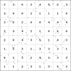
The 64 counts have mean 2.344 with standard deviation 1.5958. This gives a coefficient of determination of 1.08642, reasonably close to 1. The following table shows the expected frequencies based on a Poisson(2.344) distribution:
| Count | 0 | 1 | 2 | 3 | 4 | 5 | 6+ |
| Observed | 9 | 11 | 17 | 12 | 8 | 5 | 2 |
| Poisson | 0.096 | 0.225 | 0.264 | 0.206 | 0.121 | 0.057 | 0.032 |
| Expected | 6.1 | 14.4 | 16.9 | 13.2 | 7.7 | 3.6 | 2.1 |
There are some discrepancies between the observed and expected counts but overall they seem quite close. We can return to this example in Chapter 22 to see if the differences are statistically significant.
12. The Normal Distribution
Exercise 1
We are assuming that the lymphocyte count, [latex]X[/latex] , for a random person has the distribution [latex]\Normal{X}{2.5 \times 10^9}{0.765 \times 10^9}[/latex]. To use the Normal distribution table we need to split the probability as
\[ \pr{2.3 \times 10^9 \le X \le 2.9 \times 10^9} = \pr{X \ge 2.3 \times 10^9} - \pr{X \ge 2.9 \times 10^9}. \]
Now
\[ \pr{X \ge 2.9 \times 10^9} = \prbig{Z \ge \frac{2.9 \times 10^9 - 2.5 \times 10^9}{0.765 \times 10^9}} = \pr{Z \ge 0.52}. \]
From Table 12.1 we have [latex]\pr{Z \ge 0.52} = 0.302[/latex] . Similarly
\[ \pr{X \ge 2.3 \times 10^9} = \prbig{Z \ge \frac{2.3 \times 10^9 - 2.5 \times 10^9}{0.765 \times 10^9}} = \pr{Z \ge -0.26}. \]
Now [latex]\pr{Z \ge -0.26} = 1 - \pr{Z \le -0.26} = 1 - \pr{Z \ge 0.26} = 1 - 0.397 = 0.603[/latex]. Together we have
\[ \pr{2.3 \times 10^9 \le X \le 2.9 \times 10^9} = 0.603 - 0.302 = 0.301. \]
Note that it would have been okay to change our units to [latex]10^9[/latex] cells/L to simplify some of these expressions.
Exercise 2
We are assuming that the copper level, [latex]X[/latex], for a random person has the distribution [latex]\Normal{X}{18.5}{3.827}[/latex]. Using Table 12.1 backwards we find we need to be around 2.325 standard errors above the mean to be in the highest 1%. Here this value is
\[ 18.5 + 2.325 \times 3.827 = 27.4 \; \mu\mbox{mol/L}. \]
Note that the exact number of standard errors can be found from the [latex]\infty[/latex] row of the t-distribution table. For a tail probability of 0.01 it gives the number of standard errors to be 2.326.
Exercise 3
The following table shows [latex]\pr{X \ge x}[/latex] where [latex]X[/latex] has the uniform distribution of female heights:
| [latex]x[/latex] | 0 | 1 | 2 | 3 | 4 | 5 | 6 | 7 | 8 | 9 |
| 150 | 1.000 | 0.975 | 0.950 | 0.925 | 0.900 | 0.875 | 0.850 | 0.825 | 0.800 | 0.775 |
| 160 | 0.750 | 0.725 | 0.700 | 0.675 | 0.650 | 0.625 | 0.600 | 0.575 | 0.550 | 0.525 |
| 170 | 0.500 | 0.475 | 0.450 | 0.425 | 0.400 | 0.375 | 0.350 | 0.325 | 0.300 | 0.275 |
| 180 | 0.250 | 0.225 | 0.200 | 0.175 | 0.150 | 0.125 | 0.100 | 0.075 | 0.050 | 0.025 |
Exercise 4
The following table shows [latex]\pr{X \ge x}[/latex]where [latex]X[/latex] has the triangular distribution of female height:
| [latex]x[/latex] | 0 | 1 | 2 | 3 | 4 | 5 | 6 | 7 | 8 | 9 |
| 150 | 1.000 | 0.999 | 0.995 | 0.989 | 0.980 | 0.969 | 0.955 | 0.939 | 0.920 | 0.899 |
| 160 | 0.875 | 0.849 | 0.820 | 0.789 | 0.755 | 0.719 | 0.680 | 0.639 | 0.595 | 0.549 |
| 170 | 0.500 | 0.451 | 0.405 | 0.361 | 0.320 | 0.281 | 0.245 | 0.211 | 0.180 | 0.151 |
| 180 | 0.125 | 0.101 | 0.080 | 0.061 | 0.045 | 0.031 | 0.020 | 0.011 | 0.005 | 0.001 |
Exercise 5
The following table shows [latex]\pr{X \ge x}[/latex]where [latex]X[/latex] has the Normal distribution of female heights ([latex]\mu = 167[/latex] and [latex]\sigma = 6.6[/latex]):
| [latex]x[/latex] | 0 | 1 | 2 | 3 | 4 | 5 | 6 | 7 | 8 | 9 |
| 150 | 0.995 | 0.992 | 0.988 | 0.983 | 0.976 | 0.965 | 0.952 | 0.935 | 0.914 | 0.887 |
| 160 | 0.856 | 0.818 | 0.776 | 0.728 | 0.675 | 0.619 | 0.560 | 0.500 | 0.440 | 0.381 |
| 170 | 0.325 | 0.272 | 0.224 | 0.182 | 0.144 | 0.113 | 0.086 | 0.065 | 0.048 | 0.035 |
| 180 | 0.024 | 0.017 | 0.012 | 0.008 | 0.005 | 0.003 | 0.002 | 0.001 | 0.001 |
Exercise 6
Box plots for each of the first three rows in Table 12.2 are shown below. The same range is used for the horizontal axis to emphasize the similarities and differences between the three plots.


Exercise 7
Let [latex]X_j[/latex] be the weight of the [latex]j[/latex]th student, with [latex]\mean{X_j} = 67.1[/latex] and [latex]\sd{X_j} = 14.08[/latex], and let [latex]X = X_1 + \cdots + X_{20}[/latex] be the combined weight of 20 students. Then
\[ \mean{X} = \mean{X_1} + \cdots + \mean{X_{20}} = 20 \times 67.1 = 1342 \mbox{ kg}. \]
Assuming independence,
\[ \var{X} = \var{X_1} + \cdots + \var{X_{20}} = 20 \times 14.08^2, \]
so [latex]\sd{X} = \sqrt{20} \times 14.08 = 62.97[/latex] kg.
We can use these values to standardize
\[ \pr{X \ge 1360} = \prbig{Z \ge \frac{1360 - 1342}{62.97}} = \pr{Z \ge 0.29} = 0.386. \]
Thus there is a 39% chance that the lift will be overloaded by 20 students.
13. Sampling Distribution of the Mean
Exercise 1
The standard deviation of the mean height of eight independent observations is
\[ \sd{\overline{X}} = \frac{\sigma}{\sqrt{n}} = \frac{7.18}{\sqrt{8}} = 2.54 \mbox{ cm}. \]
Exercise 2
The sample mean has a Normal distribution with mean [latex]\mean{\overline{X}} = \mu = 4.3[/latex] mmol/L and standard deviation
\[ \sd{\overline{X}} = \frac{\sigma}{\sqrt{n}} = \frac{0.383}{\sqrt{3}} = 0.221 \mbox{ mmol/L}. \]
Thus we have
\[ \pr{\overline{X} \ge 5.0} = \prbig{Z \ge \frac{5.0 - 4.3}{0.221}} = \pr{Z \ge 3.17}. \]
The Normal distribution table gives [latex]\pr{Z \ge 3.17} = 0.001[/latex] so the probability that the mean potassium level from the sample is more than 5.0 mmol/L is 0.1%.
Exercise 3
For the cold water tablets the means from each row of 10 observations are 26.2, 26.41, 26.06, 26.32, 25.2, 27.42, 26.66, 27.5, 26.33, and 26.21 s. The mean of these means is 26.43 s with a standard deviation of 0.663 s.
In comparison, the theoretical values are [latex]\mean{\overline{X}} = \mu = 26.43[/latex] s (which will be the same since our samples cover all the tablets) and
\[ \sd{\overline{X}} = \frac{\sigma}{\sqrt{n}} = \frac{2.49}{\sqrt{10}} = 0.787 \mbox{ s}. \]
The observed standard deviation of the sample means, 0.663, is reasonably close to this value (and certainly closer to it than to the underlying standard deviation of 2.49 s).
The results for the hot water tablets are similar.
14. Confidence Intervals
Exercise 1
One critical value for [latex]t(4)[/latex] is
\[ \pr{T_4 \ge 2.132} = 0.05. \]
The closest matching [latex]t[/latex] value in the [latex]t(4)[/latex] distribution table is [latex]t_4 = 2.13[/latex] and we see there that indeed [latex]\pr{T_4 \ge 2.13} = 0.050[/latex] (to 3 decimal places).
Exercise 2
From Table 7.1 we find that the [latex]n = 12[/latex] single women have a mean basal oxytocin level of [latex]\overline{x} = 4.429[/latex] pg/mL with standard deviation [latex]s = 0.2670[/latex] pg/mL.
With [latex]12 - 1 = 11[/latex] degrees of freedom, the critical value for a 95% confidence interval is [latex]t_{11}^{*} = 2.201[/latex]. The 95% confidence interval is then
\[ 4.429 \pm 2.201 \frac{0.2670}{\sqrt{12}} = 4.429 \pm 0.170 \mbox{ pg/mL}. \]
Thus we are 95% confident that the mean basal oxytocin level for the single women that this sample was taken from is between 4.259 pg/mL and 4.599 pg/mL.
Exercise 3
We find that the [latex]n = 60[/latex] Islanders have a mean pulse rate of [latex]\overline{x} = 68.5[/latex] bpm with standard deviation [latex]s = 10.77[/latex] bpm.
With [latex]60 - 1 = 59[/latex] degrees of freedom, the critical value for a 95% confidence interval is [latex]t_{59}^{*} \approx 2.000[/latex]. (There is no row for [latex]\mbox{df} = 59[/latex] in the table so we have used the value for [latex]\mbox{df} = 60[/latex] instead. The correct value from software is [latex]t_{59}^{*} = 2.001[/latex].) The 95% confidence interval is then
\[ 68.5 \pm 2.000 \frac{10.77}{\sqrt{60}} = 68.5 \pm 2.8 \mbox{ bpm}. \]
Thus we are 95% confident that the mean pulse rate for the Islanders that this sample was taken from is between 65.7 bpm and 71.3 bpm.
15. Decisions
Exercise 1
Let [latex]\mu[/latex] be the mean passage time of light measured by Newcomb's apparatus. We want to test whether the apparatus is systematically giving a result different to the currently accepted value of 33.02. Thus we want to test [latex]H_0: \mu = 33.02[/latex] against the alternative [latex]H_1: \mu \ne 33.02[/latex].
For all [latex]n=66[/latex] observations we have [latex]\overline{x} = 26.21[/latex] and [latex]s = 10.745[/latex]. Our test statistic is then
\[ t_{66-1} = \frac{26.21 - 33.02}{10.745/\sqrt{66}} = -5.15. \]
The two-sided [latex]P[/latex]-value is [latex]2\pr{T_{65} \ge 5.15}[/latex]. From the table we see that this will be less than [latex]2 \times 0.0001 = 0.0002[/latex], substantial evidence that the apparatus was biased overall.
However, as discussed in Chapter 6, the initial observations in the data may not be as reliable as later measurements. It may be this that has resulted in the significant evidence of bias. To be fair to Newcomb we could drop the first 15 observations and work with the remaining [latex]n = 51[/latex] observations. We now find a mean of [latex]\overline{x} = 27.98[/latex] so the estimate is closer to the true value. However the standard deviation is now [latex]s = 4.798[/latex] and so the [latex]t[/latex] statistic,
\[ t_{51-1} = \frac{27.98 - 33.02}{4.798/\sqrt{51}} = -7.50, \]
actually gives stronger evidence of bias than before! The extra variability of the unusual observations was really diluting our ability to detect the bias.
Exercise 2
Let [latex]\mu[/latex] be the mean ratio of height to forearm length for the Islanders. We want to test [latex]H_0: \mu = 6[/latex] against the alternative [latex]H_1: \mu \ne 6[/latex].
A box plot for the [latex]n = 60[/latex] ratios shows that a mean of 6 seems quite unlikely.

For a t-test we find [latex]\overline{x} = 6.87[/latex] and [latex]s = 0.2804[/latex]. Our test statistic is then
\[ t_{60-1} = \frac{6.87 - 6}{0.2804/\sqrt{60}} = 24.045. \]
The corresponding two-sided [latex]P[/latex]-value will be close to 0 giving very strong evidence that the height-to-forearm ratio for the Islanders is not 6.
Exercise 3
If the mean increase is 0 then the null hypothesis is actually true. The probability of detecting this "difference" is thus the probability of rejecting the null hypothesis when it is true. This is the significance level, [latex]\alpha[/latex], and here we have [latex]\alpha = 0.05[/latex].
Exercise 4
To detect an increase of [latex]\mu = 2[/latex] when [latex]\sigma = 3[/latex] we have a signal-to-noise ratio of [latex]\frac{2}{3} = 0.67[/latex]. We can use the figure to estimate the sample size using the dashed (one-sided test) line. The result is a sample size of [latex]n=15[/latex]. (The exact value from software is [latex]n = 15.36[/latex].)
Exercise 5
Let [latex]\mu[/latex] be the mean additional hours of sleep provided by substance 2 over substance 1. We want to test [latex]H_0: \mu = 0[/latex] against [latex]H_1: \mu > 0[/latex].
For the [latex]n = 10[/latex] subjects we find a mean of [latex]\overline{x} = 1.58[/latex] additional hours of sleep with standard deviation [latex]s = 1.2300[/latex] hours. The [latex]P[/latex]-value is
\[ \pr{\overline{X} \ge 1.58} = \prbig{T_9 \ge \frac{1.58 - 0}{1.2300/\sqrt{10}}} = \pr{T_9 \ge 4.06}. \]
From the table, we find this probability is between 0.005 and 0.001. This gives strong evidence against [latex]H_0[/latex], suggesting that substance 2 does tend to give more additional hours of sleep than substance 1.
16. Comparing Two Means
Exercise 1
A box plot comparing the dye uptake shows that both distributions are reasonably symmetric and free of outliers so that we can use the [latex]t[/latex] method for calculating the confidence interval.

For the [latex]n_1 = 20[/latex] uncoated leaves we have [latex]\overline{x}_1 = 143.80[/latex] and [latex]s_1 = 11.0244[/latex] while for the [latex]n_2 = 20[/latex] coated leaves we have [latex]\overline{x}_2 = 103.55[/latex] and [latex]s_2 = 10.6449[/latex]. With minimum degrees of freedom, the critical [latex]t[/latex] value for 95% confidence is [latex]t_{19}^{*} = 2.093[/latex]. Thus the confidence interval is
\[ (143.80 - 103.55) \pm 2.093 \sqrt{ \frac{11.0244^2}{20} + \frac{10.6449^2}{20} } = 40.25 \pm 7.17 \mbox{ mm}. \]
We are 95% confident that coating the leaves with petroleum jelly reduces the mean dye uptake by between 33.08 mm and 47.42 mm.
(Using the Welch degrees of freedom from software, [latex]\mbox{df } = 37.95[/latex], gives a slightly narrower interval.)
Exercise 2
A box plot comparing the change in reaction time shows that both distributions are reasonably symmetric and free of outliers so that we can use the [latex]t[/latex]method for calculating the confidence interval. However the variability seems quite different between the groups so that a pooled method would not be appropriate.

For the [latex]n_1 = 8[/latex] males with caffeine we have [latex]\overline{x}_1 = 6.601[/latex] and [latex]s_1 = 0.4083[/latex] while for the [latex]n_2 = 8[/latex] males with decaffeinated cola we have [latex]\overline{x}_2 = 6.478[/latex] and [latex]s_2 = 1.0154[/latex]. With minimum degrees of freedom, the critical [latex]t[/latex] value for 95% confidence is [latex]t_{7}^{*} = 2.365[/latex]. Thus the confidence interval is
\[ (6.601 - 6.478) \pm 2.365 \sqrt{ \frac{0.4083^2}{8} + \frac{1.0154^2}{8} } = 0.123 \pm 0.915 \mbox{ cm}. \]
We are 95% confident that the difference in change in reaction time between having caffeine or not is between -0.792 cm and 1.038 cm. That is, we are 95% confident that the effect is between caffeine increasing reaction time by an extra 1.038 cm and reducing reaction time by an extra 0.792 cm. Since 0 is well within the interval we conclude that caffeine does not appear to have an effect on the change in reaction time after drinking rum and cola.
(Note that the Welch degrees of freedom from software, [latex]\mbox{df } = 9.206[/latex], are very close to the minimum degrees of freedom here since the standard deviations are so different between the groups.)
Exercise 3
A box plot comparing the reaction times shows that both distributions are reasonably symmetric. There is one female reaction time that is a little unusual but it may not have much effect since that group is quite large.

For the [latex]n_1 = 28[/latex] females we have [latex]\overline{x}_1 = 270.46[/latex] ms and [latex]s_1 = 19.5590[/latex] ms while for the [latex]n_2 = 16[/latex] males we have [latex]\overline{x}_2 = 274.00[/latex] ms and [latex]s_2 = 22.3488[/latex] ms. With minimum degrees of freedom, the critical [latex]t[/latex] value for 95% confidence is $t_{15}^{*} = 2.131$. Thus the confidence interval is
\[ (270.46 - 274.00) \pm 2.131 \sqrt{ \frac{19.5590^2}{28} + \frac{22.3488^2}{16} } = -3.54 \pm 14.28 \mbox{ ms}. \]
We are 95% confident that the mean reaction time for females is between 17.82 ms lower and 10.74 ms higher than the mean for males. Since 0 is well within the interval we conclude that there is inconclusive evidence of a difference in reaction times between males and females.
(Using the Welch degrees of freedom from software, [latex]\mbox{df } = 28.02[/latex], gives a slightly narrower interval.)
Exercise 4
Let [latex]\mu_1[/latex] and [latex]\mu_2[/latex] be the mean creativity scores for healthy volunteers taking 200 mg of modafinil and placebo, respectively. We want to test [latex]H_0: \mu_1 = \mu_2[/latex] against [latex]H_1: \mu_1 \ne \mu_2[/latex].
We could use a pooled two-sample [latex]t[/latex] test here, with pooled standard deviation
\[ s_p = \sqrt{\frac{31 \times 3.4^2 + 31 \times 3.8^2}{31 + 31}} = 3.6056. \]
We can use this to calculate the [latex]t[/latex] statistic
\[ t_{62} = \frac{(5.1 - 6.5) - 0}{3.6056 \sqrt{\frac{1}{32} + \frac{1}{32}}} = -1.55. \]
From the table we find [latex]\pr{T_{62} \le -1.55}[/latex] is between 0.10 and 0.05, giving a two-sided [latex]P[/latex]-value between 0.2 and 0.1. Thus there is no evidence that modafinil has an effect on mean creativity score.
Exercise 5
Let [latex]\mu_b[/latex] and [latex]\mu_g[/latex] be the mean hours of weekday television watched by boys and girls, respectively. We want to test [latex]H_0: \mu_b = \mu_g[/latex] against [latex]H_1: \mu_b \ne \mu_g[/latex].
We can again use a pooled two-sample [latex]t[/latex] test here, with pooled standard deviation
\[ s_p = \sqrt{\frac{522 \times 0.86^2 + 494 \times 0.88^2}{522 + 494}} = \sqrt{0.7565} = 0.8698 \]
We can use this to calculate the [latex]t[/latex] statistic
\[ t_{1016} = \frac{(2.42 - 2.24) - 0}{0.8698 \sqrt{\frac{1}{523} + \frac{1}{495}}} = 3.30. \]
From Table 14.2 we find [latex]\pr{T_{1016} \ge 3.30}[/latex] is roughly 0.0005, giving a two-sided [latex]P[/latex]-value of around 0.001. Thus there is strong evidence that the mean hours of weekday television watched is different between boys and girls.
Exercise 6
Let [latex]\mu_r[/latex] and [latex]\mu_d[/latex] be the mean durations produced by rested and sleep deprived subjects, respectively. We want to test [latex]H_0: \mu_r = \mu_d[/latex] against [latex]H_1: \mu_r \ge \mu_d[/latex].
From the [latex]n_r = 5[/latex] rested observations we find [latex]\overline{x}_r = 1591[/latex] ms ([latex]s_r = 189.5[/latex] ms) while for the [latex]n_d = 5[/latex] sleep deprived observations we find [latex]\overline{x}_d = 1270[/latex] ms ([latex]s_d = 257.6[/latex] ms). We can use these to calculate the [latex]t[/latex] statistic
\[ t_4 = \frac{(1591 - 1270) - 0}{\sqrt{\frac{189.5^2}{5} + \frac{257.6^2}{5}}} = 2.24, \]
where we have use the conservative degrees of freedom [latex]\mbox{df } = \min(n_r - 1, n_d -1) = 4[/latex].
From the table we find that the [latex]P[/latex]-value [latex]\pr{T_4 \ge 2.24}[/latex] is between 0.05 and 0.025, giving some evidence that the mean duration produced is lower for sleep deprived subjects.
Exercise 7
Let [latex]\mu_1[/latex] and [latex]\mu_2[/latex] be the mean total number of plant species present in organic and conventional vineyards, respectively. We want to test [latex]H_0: \mu_1 = \mu_2[/latex] against [latex]H_1: \mu_1 \ge \mu_2[/latex].
We can use the given summary values to calculate the [latex]t[/latex] statistic
\[ t_8 = \frac{(31.1 - 26.6) - 0}{\sqrt{\frac{5.21^2}{9} + \frac{1.96^2}{11}}} = 2.45, \]
where we have use the conservative degrees of freedom [latex]\mbox{df } = \min(n_1 - 1, n_2 -1) = 8[/latex].
From the table we find that the \pv-value [latex]\pr{T_8 \ge 2.45}[/latex] is between 0.025 and 0.01, giving moderate evidence that the mean total number of plant species is higher in organic vineyards.
Note that this result should be taken with some caution since the fifth vineyard has a very high species count, as seen in the following box plot:

Should we be concerned? Dropping that value reduces the mean total species for organic vineyards from 31.1 to 29.75, though it also reduces the standard deviation from 5.21 to 3.45. The revised [latex]t[/latex] statistic would be
\[ t_7 = \frac{(29.75 - 26.6) - 0}{\sqrt{\frac{3.45^2}{8} + \frac{1.96^2}{11}}} = 2.32, \]
with the [latex]P[/latex]-value [latex]\pr{T_7 \ge 2.32}[/latex] now slightly above 0.025, but with a similar conclusion as before.
17. Inferences for Proportions
Exercise 1
We now want to look through Table 11.4 at the [latex]p = 0.50[/latex] column to find the first [latex]n[/latex]such that there is a two-sided probability less than 0.05. For [latex]n=5[/latex] we have [latex]\pr{X \ge 5} = 0.031[/latex] so this is not quite small enough. However for [latex]n=6[/latex] we have [latex]\pr{X \ge 6} = 0.016[/latex]. Thus if we toss a coin 6 times and observe 6 heads or 6 tails then we could reject the null hypothesis that [latex]p = 0.5[/latex].
The power of this procedure is then the probability of actually observing 6 heads or tails for the true value of [latex]p[/latex]. From the Binomial formula this is
\[ \pr{X = 0} + \pr{X = 6} = {6 \choose 0} p^0 (1-p)^6 + {6 \choose 6} p^6 (1-p)^0 = (1-p)^6 + p^6, \]
and we want to find [latex]p[/latex]such that this power is 0.80. One way to solve this is using fixed-point iteration. We can rearrange the equation we want to solve as
\[ p = \sqrt[6]{0.8 - (1-p)^6}. \]
Pick a starting value, such as [latex]p = 0.5[/latex] and substitute into the right-hand side to get a new value of [latex]p[/latex]. Repeating this gives
\[ p = 0.5 \rightarrow 0.96033 \rightarrow 0.963492, \]
after which the answer doesn't change to 6 decimal places, giving one solution for a power of 80% to be [latex]p = 0.96[/latex].
Thus if the actually probability of heads (or tails) is 96% or higher then we will observe 6 or 0 heads at least 80% of the time. This essentially means that the only way we will detect bias with 80% power through 6 coin tosses is if the coin actually has heads (or tails) on both sides.
Exercise 2
The continuity correction uses
\[ \pr{X = 10} = \pr{9.5 \le X \le 10.5} \]
which is a true identity for discrete [latex]X[/latex]. We have [latex]\mean{X} = 15 \times 0.4 = 6[/latex] and [latex]\sd{X} = \sqrt{15 \times 0.4 \times 0.6} = 1.897[/latex]. The Normal approximation gives
\[ \pr{X \ge 10.5} \approx \prbig{Z \ge \frac{10.5 - 6}{1.897}} = \pr{Z \ge 2.37} = 0.009. \]
Similarly
\[ \pr{X \ge 9.5} \approx \prbig{Z \ge \frac{9.5 - 6}{1.897}} = \pr{Z \ge 1.84} = 0.033, \]
so [latex]\pr{9.5 \le X \le 10.5} \approx 0.033 - 0.009 = 0.024[/latex]. This is actually the same value as given in the Binomial distribution table (to three decimal places).
Exercise 3
Assuming the sample size will be reasonably large, the Normal approximation gives a margin of error of
\[ m = 1.960 \sqrt{\frac{p(1-p)}{n}}. \]
To solve this we need an estimate of [latex]p[/latex]. The most conservative value to choose is [latex]p = 0.5[/latex] since this gives the largest value of [latex]p(1-p)[/latex] and hence the worst case scenario for the resulting margin of error. We then have
\[ 0.04 = 1.960 \sqrt{\frac{0.25}{n}} \Rightarrow n = \frac{1.960^2 \times 0.25}{0.04^2} = 600.25. \]
Thus we will need a sample size of around 600 (at most) to obtain a margin of error of 4%.
Exercise 4
This is similar to the previous exercise except that now we know we are particularly interested in values of [latex]p[/latex] around 0.05. We can use this to estimate margin of error (instead of the conservative [latex]p=0.5[/latex]). Thus
\[ 0.005 = 1.960 \sqrt{\frac{0.05(0.95)}{n}} \Rightarrow n = \frac{1.960^2 \times 0.0475}{0.005^2} = 7299. \]
Thus we will need around 7300 randomizations to obtain a [latex]P[/latex]-value around 5% correct to within a 95% margin of error of 0.5%.
Exercise 5
The proportion of Islanders in the sample who said Yes is 43/60 = 0.717. The margin of error for a 95% confidence interval is then
\[ 1.96\sqrt{\frac{0.717 \times (1 - 0.717)}{60}} = 0.114, \]
so we are 95% confident that the proportion of Islanders who would say Yes is [latex]0.717 \pm 0.114[/latex], or between 60.3% and 83.1%.
Exercise 6
Let [latex]q[/latex] be the proportion of students who would say Yes to the question (the value estimated by the confidence interval in Exercise 5) and let [latex]p[/latex] be the proportion of students who do actually approve of kissing on the first date. In Chapter 9 we saw that
\[ q \approx 0.25 + 0.5p \]
and we can rearrange this to get an estimate of [latex]p[/latex] given an estimate of [latex]q[/latex]. From Exercise 5 we have an estimate for the upper limit of [latex]q[/latex] of 0.831 which gives an estimate for the upper limit for [latex]p[/latex] of [latex]2(0.831 - 0.25) = 1.162[/latex]. Similarly a lower limit for [latex]p[/latex] is [latex]2(0.603 - 0.25) = 0.706[/latex].
How can the upper limit be 1.162 when proportions have to be between 0 and 1? The reason is because we are using a Normal approximation to the proportions in our calculations and Normal distributions do not have bounds on their range and this will particularly be an issue for small sample sizes. Here we could just say that the upper limit for [latex]p[/latex] is 1.
Exercise 7
We can summarize the data in a two-way table:
| Aspirin | Placebo | |
| Cancer Death | 75 | 47 |
| No Cancer Death | 3354 | 1663 |
| Total | 3429 | 1710 |
The odds ratio of death due to cancer between the aspirin and control groups is
\[ \mbox{OR } = \frac{75/3354}{47/1663} = 0.7912. \]
By taking logarithms, we can use the Normal distribution to calculate a [latex]P[/latex]-value to determine whether this is significantly different from a null ratio of 1. Here
\[ \ln(\mbox{OR}) = \ln(0.7912) = -0.2342 \]
with
\[ \se{\ln(\mbox{OR})} = \sqrt{\frac{1}{75} + \frac{1}{47} + \frac{1}{3354} + \frac{1}{1663}} = 0.1884. \]
If the null hypothesis is true then we would expect [latex]\ln(\mbox{OR}) = 0[/latex]. We can test this using the [latex]z[/latex] statistic
\[ z = \frac{-0.2342 - 0}{0.1884} = -1.24. \]
Since we are interested in the odds being lower for aspirin, the one-sided [latex]P[/latex]-value is [latex]\pr{Z \le -1.24} = 0.107[/latex]. Thus there is no evidence that aspirin has lowered the odds of death due to cancer.
18. Inferences for Regression
Exercise 1
Software can be used to obtain the following regression summary:
| Estimate | SE | T | P | |
| Constant | -181.7405 | 59.2889 | -3.065 | 0.00667 |
| Height | 1.2774 | 0.3388 | 3.770 | 0.00140 |
The [latex]P[/latex]-value associated with the test of a zero slope is 0.00140, very strong evidence to suggest an association between time breath can be held and the height of the subject. The relationship can be seen in the following scatter plot:

Exercise 2
For males we find the following regression summary:
| Estimate | SE | T | P | |
| Constant | 42.58453 | 103.36221 | 0.412 | 0.691 |
| Height | 0.07815 | 0.56826 | 0.138 | 0.894 |
The relationship still seems positive but now the [latex]P[/latex]-value associated with the test of a zero slope is 0.894, no evidence of an association between time breath can be held and the height of the subject.
For females we obtain:
| Estimate | SE | T | P | |
| Constant | 84.3331 | 71.5403 | 1.179 | 0.272 |
| Height | -0.3468 | 0.4264 | -0.813 | 0.440 |
The relationship for females is actually negative though again we find no evidence of a slope different to 0.
So why do we find a strong association for all subjects but then no association for males or for females separately? The reason can be seen in an updated scatter plot where we have split the subjects according to sex.

There does appear to be no association overall. The spurious result in Exercise 1 arose because the best line to fit the data joined the group of female observation in the bottom left with the male observations in the top right, giving a significant positive slope to the line. This highlights why it is important to look for confounding variables when coming to conclusions.
Exercise 3
From software we find that the correlation coefficient is [latex]r = 0.5819[/latex] from the [latex]n=60[/latex] subjects (where we have corrected the unusual forearm value). This suggests a strong positive association between height and forearm length.
To carry out a test of [latex]H_0: \rho = 0[/latex] against [latex]H_1: \rho \ne 0[/latex] we use the [latex]t[/latex] statistic
\[ t_{58} = \frac{0.5819 - 0}{\sqrt{\frac{1 - 0.5819^2}{58}}} = 5.45. \]
The corresponding [latex]P[/latex]-value will be close to 0, giving strong evidence of an association.
Exercise 4
We can use Fisher's [latex]Z[/latex] transformation to calculate a confidence interval for [latex]\rho[/latex] based on the observed [latex]r = 0.5819[/latex]. Firstly we use the inverse hyperbolic tangent function to obtain
\[ z = \mbox{arctanh}(0.5819) = 0.6653. \]
This value has standard error
\[ \se{z} = \sqrt{\frac{1}{60 - 3}} = 0.1325, \]
giving a 95% confidence interval for [latex]z[/latex] of
\[ 0.6653 \pm 1.96 \times 0.1325 = 0.6653 \pm 0.2596, \]
or [latex](0.4057, 0.9249)[/latex].
To convert this into a confidence interval for [latex]\rho[/latex] we apply the hyperbolic tangent function to each end of this interval, finding [latex]\tanh(0.4057) = 0.3848[/latex] and [latex]\tanh(0.9249) = 0.7282[/latex]. Thus we are 95% confident that the correlation between height and forearm length for the Islanders is between around 0.38 and 0.73.
Exercise 5
Let [latex]\rho[/latex] be the underlying correlation between total plant species and years of organic management. We want to test [latex]H_0: \rho = 0[/latex] against [latex]H_1: \rho > 0[/latex].
Based on the observed correlation, we can test [latex]H_0[/latex] using the [latex]t[/latex] statistic
\[ t_{9-2} = \frac{0.7060 - 0}{\sqrt{\frac{1 - 0.7060^2}{9-2}}} = 2.64. \]
From Table 14.2, the [latex]P[/latex]-value, [latex]\pr{T_7 \ge 2.64}[/latex], is between 0.025 and 0.01. This gives moderate evidence that the total plant species tends to increase with years of organic management.
19. Analysis of Variance
Exercise 1
When [latex]n=1[/latex] the [latex]F(n,d)[/latex] distribution is the distribution of the square of a [latex]t_d[/latex] statistic. For example, one critical value in Table 19.3 is
\[ \pr{F_{1,12} \ge 4.75} = 0.05. \]
Since the squaring removes the sign, this will correspond to a two-sided probability in the [latex]t(12)[/latex] distribution. We find
\[ \pr{t_{12} \ge 2.179} = 0.025, \]
and indeed [latex]2.179^2 = 4.748[/latex].
Exercise 2
A side-by-side dot plot shows that the three distributions are free of outliers and have similar variability:

The ANOVA table from software is
| Source | df | SS | MS | F | P |
| Storage | 2 | 4249.7 | 2124.87 | 17.881 | 0.0002515 |
| Residuals | 12 | 1426.0 | 118.83 | ||
| Total | 14 | 5675.7 |
The F-test thus gives strong evidence of a difference between the three means.
Note that the test does not say anything about the nature of the difference. From the plot it appears that the Water and Bag storage methods gave similar results. The question of how to make these subsequent comparisons is addressed in Chapter 20.
Exercise 3
With 537 subjects the total degrees of freedom are 536, while with 3 consumption groups the Green Tea degrees of freedom are 2, leaving 534 for residuals. The mean sums of squares are then [latex]\frac{64.42}{2} = 32.21[/latex] and [latex]\frac{5809.64}{534} = 10.879[/latex], giving the [latex]F[/latex] statistic
\[ F_{2,534} = \frac{32.21}{10.879} = 2.961. \]
The completed ANOVA table is shown below. The [latex]P[/latex]-value is [latex]\pr{F_{2,534} \ge 2.961}[/latex] and from the table we find this is just above 0.05, inconclusive evidence of a difference in mean BMI between the three groups.
| Source | df | SS | MS | F | P |
| Green Tea | 2 | 64.42 | 32.21 | 2.961 | > 0.05 |
| Residuals | 534 | 5809.64 | 10.879 | ||
| Total | 536 | 5873.83 |
Exercise 4
- The pooled residual sum of squares is
\[ (207-1) \times 11.8^2 + (114-1) \times 11.2^2 + (216-1) \times 10.0^2 = 64358 \]
with degrees of freedom [latex](207-1) + (114-1) + (216-1) = 534[/latex]. - The three totals are [latex]T_1 = 207 \times 42.0 = 8694[/latex], [latex]T_2 = 114 \times 43.7 = 4982[/latex]and [latex]T_3 = 216 \times 46.2 = 9979[/latex], giving grand total [latex]T = 23655[/latex].
- This gives
\[ \mbox{SSG } = \frac{8694^2}{207} + \frac{4982^2}{114} + \frac{9979^2}{216} - \frac{23655^2}{537} = 1881. \] - We can use these values to construct the following ANOVA table:
Source df SS MS F P Coffee 2 1881 940.5 7.804 ≈ 0.001 Residuals 534 64358 120.5 Total 536 66239 From the tables, the [latex]P[/latex]-value is approximately 0.001, giving strong evidence of a difference in mean age between the three coffee consumption groups.
20. Multiple Comparisons
Exercise 1
The ANOVA table from software is
| Source | df | SS | MS | F | P |
| Wingspan | 2 | 16093 | 8046.4 | 3.0959 | 0.06159 |
| Residuals | 27 | 70175 | 2599.1 | ||
| Total | 29 | 86268 |
This F-test gives weak evidence ([latex]p = 0.06[/latex]) of a difference in mean flight distance between the three wingspans.
The pooled standard deviation is [latex]\sqrt{\mbox{MSE}} = \sqrt{2599.1} = 50.98[/latex] cm. For 95% Bonferroni intervals based on the three comparisons we would use
\[ \alpha = \frac{0.05}{3} = 0.017. \]
We thus calculate 98.3% confidence intervals based on the differences and using the pooled estimate of standard deviation.
The mean distances flown for the 6, 4 and 2 cm wingspans are 245.8, 256.5 and 299.4 cm, respectively.
The critical [latex]t_{27}[/latex] value required for 98.3% confidence is not available in the table and we don't have a table for the [latex]t(27)[/latex] distribution. However, from software we find the critical value needed is [latex]t_{27}^{*} = 2.552[/latex] since [latex]\pr{T_{27} \ge 2.552} = \frac{0.017}{2}[/latex].
The interval for comparing the 6 cm wingspan with the 4 cm wingspan is thus
\begin{align*}
(245.8 - 256.5) \pm 2.552 \sqrt{\frac{50.98^2}{10} + \frac{50.98^2}{10}} & = -10.7 \pm 2.552 \times 50.98 \sqrt{\frac{2}{10}} \\
& = -10.7 \pm 58.2.
\end{align*}
The other two intervals have the same margins of error (since the samples all had the same size).
It is always important to visualize the data to check the assumptions underlying these methods. This scatter plot includes a line joining the three means together.

The distributions within each wingspan seem reasonably symmetric but there does seem to be differences in the variability between the groups. One consequence of this is that using a pooled standard deviation in our confidence interval will overestimate errors if the 2 cm planes are being compared and will underestimate errors if the 6 cm planes are being compared.
Exercise 2
The ANOVA table for the regression analysis is
| Source | df | SS | MS | F | P |
| Wingspan | 1 | 14365 | 14364.8 | 5.5939 | 0.02519 |
| Residuals | 28 | 71903 | 2567.9 | ||
| Total | 29 | 86268 |
We now find some moderate evidence of a wingspan effect, even though the residual error is similar to that in Exercise 20.1. The reason for this is that we are adding the extra information to the model that we have a linear relationship. With stronger assumptions we can make stronger inferences from the same amount of information. It is very important then to validate whether this assumption is appropriate. The scatter plot below now has the regression line included.

This does not seem a terribly plausible model for the data, especially in the presence of the variability in the 6 cm group. We should thus treat the results of this analysis with some caution.
Exercise 3
The HSD was 105.9 lbs and looking through Table 20.3 we find the following pairwise differences to be larger than this value:
| Pair | Difference |
| A - C | -132.8 |
| A - E | -175.2 |
| A - F | -256.8 |
| B - F | -175.3 |
| C - F | -124.0 |
| D - E | -115.0 |
| D - F | -196.7 |
These correspond exactly to the pairwise [latex]P[/latex]-values that were less than 5% in Table 20.7.
Exercise 4
From Table 19.8, the pairwise differences (mL) are
| Pair | Difference |
| Low - None | 2.7 |
| High - None | 4.6 |
| High - Low | 1.9 |
From Table 19.9, the pooled standard deviation is [latex]\sqrt{1.042} = 1.0208[/latex] with 12 degrees of freedom. The critical [latex]t[/latex] value is 2.179, giving the LSD
\[ 2.179 \times 1.0208 \sqrt{\frac{1}{5} + \frac{1}{5}} = 1.41 \mbox{ mL}. \]
Thus all three pairwise comparisons are found to be significant by the LSD.
The critical value for the HSD is [latex]q^{*}_{3,12} = 3.77[/latex], from Table 20.8. This gives the HSD
\[ 3.77 \frac{1.0208}{\sqrt{5}} = 1.72 \mbox{ mL}. \]
This is higher than the LSD, as expected, but all three pairwise comparisons are still found to be significant.
21. Multiple Regression
Exercise 1
Software can be used to obtain the following regression summary:
| Estimate | SE | T | P | |
| Constant | 49.8795 | 17.9115 | 2.785 | 0.007 |
| Forearm | 4.6446 | 0.7072 | 6.567 | < 0.001 |
| SexMale | 14.5428 | 22.2086 | 0.655 | 0.515 |
| Forearm:SexMale | -0.1550 | 0.8795 | -0.176 | 0.861 |
The seems to be no interaction between forearm length and sex on the height values ([latex]p = 0.861[/latex]) and so we could drop this from our model. Looking for a parallel relationship between height and forearm length for males and females gives
| Estimate | SE | T | P | |
| Constant | 52.4155 | 10.5712 | 4.958 | < 0.001 |
| Forearm | 4.5444 | 0.4168 | 10.903 | < 0.001 |
| SexMale | 10.6330 | 0.9277 | 11.462 | < 0.001 |
There is now strong evidence of a difference between males and females, with males tending to be on average 10.63 cm taller than females for the same forearm length.
Exercise 2
The regression summary is:
| Estimate | SE | T | P | |
| Constant | 63.86929 | 20.61941 | 3.098 | 0.00452 |
| Weight | 0.13886 | 0.07354 | 1.888 | 0.06979 |
| TreatmentNone | 7.02763 | 4.52686 | 1.552 | 0.13220 |
There is weak evidence of an association between the juice obtained and orange weight ([latex]p = 0.06979[/latex]) but there is no evidence of a treatment effect.
Exercise 3
The [latex]R^2[/latex] value is
\[ R^2 = \frac{0.0155}{2.0828} = 0.0074. \]
The adjusted [latex]R^2[/latex] value is then
\[ \overline{R}^2 = 1 - (1 - 0.0074)\frac{23}{22} = -0.0377. \]
This is negative (since the [latex]R^2[/latex] value was so small) and highlights that the adjusted [latex]R^2[/latex] cannot be interpreted as a proportion.
Exercise 4
With 36 plots, the total degrees of freedom are 35. There were 3 phosphate levels, giving 2 degrees of freedom for the phosphate factor. Similarly there were 2 nitrogen levels so there is 1 degree of freedom for nitrogen. The degrees of freedom for an interaction effect are thus [latex]2 \times 1 = 2[/latex], leaving 30 residual degrees of freedom. We can use these to complete the following table:
| Source | df | SS | MS | F | P |
| Phosphate | 2 | 164872 | 82436 | 22.6 | < 0.001 |
| Nitrogen | 1 | 77191 | 77191 | 21.2 | < 0.001 |
| Interaction | 2 | 6117 | 3059 | 0.84 | > 0.1 |
| Residuals | 30 | 109207 | 3640 | ||
| Total | 35 | 357387 |
We thus have strong evidence of phosphate and nitrogen effects on potato yield but no evidence of an interaction between the two.
22. Contingency Tables
Exercise 1
As in Table 22.2, with 900 digits we would expect to see each digit [latex]\frac{900}{10} = 90[/latex] times. The table below shows the observed counts:
| Digit | 0 | 1 | 2 | 3 | 4 | 5 | 6 | 7 | 8 | 9 |
| Observed | 87 | 117 | 67 | 40 | 170 | 94 | 101 | 113 | 61 | 50 |
| Expected | 90 | 90 | 90 | 90 | 90 | 90 | 90 | 90 | 90 | 90 |
The [latex]\chi^2[/latex] statistic is
\[ \chi^2 = \frac{(87 - 90)^2}{90} + \frac{(117 - 90)^2}{90} + \cdots + \frac{(50 - 90)^2}{90} = 147.5. \]
With 10 outcomes we have [latex]10 - 1 = 9[/latex] degrees of freedom and so the [latex]P[/latex]-value is [latex]\pr{\chi_9^2 \ge 147.5}[/latex]. From Table 22.4, this is less than 0.001, substantial evidence that the second batch of human random digits are not uniformly distributed either.
Exercise 2
With 1800 digits we would expect to see each digit [latex]\frac{1800}{10} = 180[/latex] times. The table below shows the observed counts:
| Digit | 0 | 1 | 2 | 3 | 4 | 5 | 6 | 7 | 8 | 9 |
| Observed | 176 | 165 | 185 | 184 | 184 | 170 | 184 | 184 | 180 | 188 |
| Expected | 180 | 180 | 180 | 180 | 180 | 180 | 180 | 180 | 180 | 180 |
The [latex]\chi^2[/latex] statistic is
\[ \chi^2 = \frac{(176 - 180)^2}{180} + \frac{(165 - 180)^2}{180} + \cdots + \frac{(188 - 180)^2}{180} = 2.74. \]
With 10 outcomes we have [latex]10 - 1 = 9[/latex] degrees of freedom and so the [latex]P[/latex]-value is [latex]\pr{\chi_9^2 \ge 2.74}[/latex]. From Table 22.4, this is greater than 0.95, no evidence to suggest that the digits of [latex]e[/latex] are not uniformly distributed.
Exercise 3
With 1800 digits we would expect to see each digit [latex]\frac{1800}{10} = 180[/latex] times. The table below shows the observed counts:
| Digit | 0 | 1 | 2 | 3 | 4 | 5 | 6 | 7 | 8 | 9 |
| Observed | 162 | 195 | 186 | 173 | 175 | 188 | 173 | 178 | 180 | 190 |
| Expected | 180 | 180 | 180 | 180 | 180 | 180 | 180 | 180 | 180 | 180 |
The [latex]\chi^2[/latex] statistic is
\[ \chi^2 = \frac{(162 - 180)^2}{180} + \frac{(195 - 180)^2}{180} + \cdots + \frac{(190 - 180)^2}{180} = 4.87. \]
With 10 outcomes we have [latex]10 - 1 = 9[/latex] degrees of freedom and so the [latex]P[/latex]-value is [latex]\pr{\chi_9^2 \ge 4.87}[/latex]. From Table 22.4, this is greater than 0.25, no evidence to suggest that the digits of [latex]\pi[/latex] are not uniformly distributed.
Exercise 4
With 120 rolls we would expect to see each die outcome [latex]\frac{120}{6} = 20[/latex] times. The table below shows the observed counts:
| Outcome | 1 | 2 | 3 | 4 | 5 | 6 |
| Observed | 16 | 22 | 18 | 12 | 32 | 20 |
| Expected | 20 | 20 | 20 | 20 | 20 | 20 |
The [latex]\chi^2[/latex]statistic is
\[ \chi^2 = \frac{(16 - 20)^2}{20} + \frac{(22 - 20)^2}{20} + \cdots + \frac{(20 - 20)^2}{20} = 11.6. \]
With 6 outcomes we have [latex]6 - 1 = 5[/latex] degrees of freedom and so the [latex]P[/latex]-value is [latex]\pr{\chi_5^2 \ge 11.6}[/latex]. From Table 22.4, this is somewhere between 0.05 and 0.025, some evidence that the dice outcomes at Mossgiel are unusual.
Exercise 5
The observed and expected counts from the solution to Exercise 11.9 are
| Count | 0 | 1 | 2 | 3 | 4 | 5 | 6+ |
| Observed | 9 | 11 | 17 | 12 | 8 | 5 | 2 |
| Poisson | 0.096 | 0.225 | 0.264 | 0.206 | 0.121 | 0.057 | 0.032 |
| Expected | 6.1 | 14.4 | 16.9 | 13.2 | 7.7 | 3.6 | 2.1 |
The [latex]\chi^2[/latex] statistic is
\[ \chi^2 = \frac{(9 - 6.1)^2}{6.1} + \frac{(11 - 14.4)^2}{14.4} + \cdots + \frac{(2 - 2.1)^2}{2.1} = 2.85. \]
With 7 groups and an unknown parameter ([latex]\lambda[/latex]) we have [latex]7 - 1 - 1= 5[/latex] degrees of freedom and so the [latex]P[/latex]-value is [latex]\pr{\chi_5^2 \ge 2.85}[/latex]. From Table 22.4, this is greater than 0.25, no evidence to suggest that the distribution is not Poisson.
Exercise 6
The observed counts for pizza preference by region are given in the following table.
| Mushroom | Pineapple | Prawns | Sausage | Spinach | Total | |
| Ironbard | 28 | 49 | 30 | 49 | 44 | 200 |
| Providence | 43 | 41 | 28 | 44 | 44 | 200 |
| Total | 71 | 90 | 58 | 93 | 88 | 400 |
The expected counts if the two variables were independent are
| Mushroom | Pineapple | Prawns | Sausage | Spinach | Total | |
| South | 35.5 | 45.0 | 29.0 | 46.5 | 44.0 | 200 |
| North | 35.5 | 45.0 | 29.0 | 46.5 | 44.0 | 200 |
| Total | 71 | 90 | 58 | 93 | 88 | 400 |
The [latex]\chi^2[/latex] statistic is then
\[ \chi^2 = \frac{(28 - 35.5)^2}{35.5} + \frac{(49 - 45.0)^2}{45.0} + \cdots + \frac{(44 - 44.0)^2}{44.0} = 4.22. \]
With 2 rows and 5 columns we have [latex](2 - 1) \times (5-1) = 4[/latex] degrees of freedom and so the [latex]P[/latex]-value is [latex]\pr{\chi_4^2 \ge 4.22}[/latex]. From Table 22.4, this is greater than 0.25, giving no evidence of a difference in pizza preference between the two islands.
Exercise 7
The non-smokers have a large number of women in the 65+ age group. Mortality is naturally high in this group anyway and so overall the rate of death for non-smokers appears higher. That is, it is actually because smokers don't live so long that the overall mortality of smokers appears lower!
Exercise 8
Calculating the marginal totals gives
| Age group | Under 18 | 18-25 | 26-40 | Over 40 | Total |
| Interested | 136 | 42 | 48 | 75 | 301 |
| Not interested | 83 | 18 | 31 | 17 | 149 |
| Total | 219 | 60 | 79 | 92 | 450 |
Assuming age group and interest in green roof systems are independent, we can calculate expected values such as
\[ \frac{301}{450} \times \frac{219}{450} \times 450 = \frac{301 \times 219}{450} = 146.5 \]
for the number of under 18's interested in green roof systems. Calculating the other 7 values gives the table of expected values
| Age group | Under 18 | 18-25 | 26-40 | Over 40 |
| Interested | 146.5 | 40.1 | 52.8 | 61.5 |
| Not interested | 72.5 | 19.9 | 26.2 | 30.5 |
The [latex]\chi^2[/latex] statistic to compare the observed counts with these expected counts is
\[ \frac{(136 - 146.5)^2}{146.5} + \frac{(42 - 40.1)^2}{40.1} + \cdots + \frac{(17 - 30.5)^2}{30.5} = 12.764. \]
The [latex]P[/latex]-value is [latex]\pr{\chi^2_3 \ge 12.764}[/latex], between 0.01 and 0.005 from Table 22.4. Thus there is strong evidence of an association between age group and interest in green roof systems.
23. Logistic Regression
Exercise 1
Logistic regression fits the model
\[ \ln \left( \frac{p}{1-p} \right) = b_0 + b_1 x. \]
If [latex]p = 0.5[/latex] then [latex]\frac{p}{1-p} = 1[/latex] and [latex]\ln(1) = 0[/latex]. Thus we want [latex]x[/latex] such that
\[ 0 = b_0 + b_1 x \; \Rightarrow \; x = -\frac{b_0}{b_1}. \]
Exercise 2
The logistic regression summary from software is
| Estimate | SE | Z | P | |
| Constant | -11.39669 | 7.08158 | -1.609 | 0.1075 |
| Height | 0.07165 | 0.04133 | 1.734 | 0.0829 |
The [latex]P[/latex]-value of interest is [latex]p = 0.0829[/latex], giving weak evidence of an association between responding Yes to the question about kissing on the first date and height. Note that we have found this weak evidence even though the Yes responses include a random component due to the outcome of the coin toss.
A plot showing the logistic fit is given below:

Exercise 3
Let [latex]\beta_1[/latex]be the underlying slope in the logistic relationship
\[ \ln\left(\frac{p}{1-p}\right) = \beta_0 + \beta_1 x, \]
where [latex]x[/latex] is the average hours of television watched as a child and [latex]p[/latex] is the probability of a criminal conviction by age 26. We want to test [latex]H_0: \beta_1 = 0[/latex] against [latex]H_1: \beta_1 > 0[/latex].
We estimate [latex]\beta_1[/latex] with [latex]b_1 = 0.4383[/latex]. We can test [latex]H_0[/latex] using
\[ z = \frac{0.4383 - 0}{0.1012} = 4.33. \]
The [latex]P[/latex]-value is [latex]\pr{Z \ge 4.33} \ll 0.001[/latex], very strong evidence of a positive association between the probability of a criminal conviction by age 26 and the average hours of television watched as a child.
Exercise 4
The slope in logistic regression estimates the log of the odds ratio for a one-unit increase in the explanatory variable. Here a 95% confidence interval for the slope is
\[ 0.4383 \pm 1.960 \times 0.1012 = 0.4383 \pm 0.1984, \]
or [latex](0.2399,0.6367)[/latex]. Thus we are 95% confident that a one-hour increase in average hours of television will increase odds by a factor of between [latex]e^{0.2399} = 1.27[/latex] and [latex]e^{0.6367} = 1.89[/latex].
24. Nonparametric Methods
Exercise 1
Let [latex]p[/latex] be the probability that the right hopping speed is faster than the left hopping speed and let [latex]X[/latex] be the count of this occurring. Our null hypothesis is that [latex]\Binomial{X}{11}{0.5}[/latex].
We observe [latex]X = 6[/latex] so that the one-sided [latex]P[/latex]-value is [latex]\pr{X \ge 6} = 0.5[/latex], from the Binomial table. Thus there is no evidence of a difference from a sign test.
Exercise 2
The differences and the ranked absolute differences are shown in the following table.
| Subject | 1 | 2 | 3 | 4 | 5 | 6 | 7 | 8 | 9 | 10 | 11 |
| Left | 124 | 86 | 98 | 112 | 104 | 190 | 135 | 110 | 78 | 82 | 94 |
| Right | 110 | 98 | 110 | 110 | 108 | 195 | 125 | 120 | 70 | 80 | 98 |
| R - L | -14 | 12 | 12 | -2 | 4 | 5 | -10 | 10 | -8 | -2 | 4 |
| Rank | 11 | 9.5 | 9.5 | 1.5 | 3.5 | 5 | 7.5 | 7.5 | 6 | 1.5 | 3.5 |
The signed-rank statistic is the sum of the ranks of the positive differences,
\[ S = 9.5 + 9.5 + 3.5 + 5 + 7.5 + 3.5 = 38.5. \]
Table 24.4 is based on ranks with no ties though we can still see that a score of 42 is required to obtain a one-sided [latex]P[/latex]-value less than 0.25.
For the Normal approximation, the expected value of [latex]S[/latex] is [latex]\mean{S} = \frac{11(11+1)}{4} = 33[/latex] with estimated standard deviation
\[ \sd{S} = \sqrt{\frac{11(11+1)(22+1)}{24}} = \sqrt{126.5} = 11.25. \]
(This standard deviation will be a slight over-estimate since several ranks were tied for this data.) The one-sided [latex]P[/latex]-value is then
\[ \pr{S \ge 38.5} \approx \prbig{Z \ge \frac{38.5 - 33}{11.25}} = \pr{Z \ge 0.49} = 0.312, \]
from the Normal Distribution table. Thus again there is no evidence of a difference in hopping speeds between the two legs.
Exercise 3
The weights and the ranked weights are shown in the following table.
| M | F | F | F | F | F | M | F | M | F | F | M | M | F | M |
| 74 | 67 | 68 | 53 | 65 | 59 | 52 | 60 | 72 | 72 | 59 | 62 | 100 | 58 | 79 |
| 44.5 | 33.5 | 36 | 5.5 | 30.5 | 17.5 | 4 | 21 | 42 | 42 | 17.5 | 25 | 59 | 15 | 51 |
| M | M | F | F | M | M | M | M | M | F | M | F | M | M | F |
| 81 | 55 | 45 | 72 | 64 | 59 | 65 | 71 | 60 | 57 | 62 | 77 | 68 | 81 | 54 |
| 54.5 | 10 | 1 | 42 | 28.5 | 17.5 | 30.5 | 39.5 | 21 | 12.5 | 25 | 49 | 36 | 54.5 | 8 |
| F | M | M | F | M | F | F | M | M | F | F | M | F | M | M |
| 79 | 75 | 109 | 60 | 76 | 71 | 57 | 76 | 54 | 63 | 62 | 79 | 57 | 80 | 64 |
| 51 | 46 | 60 | 21 | 47.5 | 39.5 | 12.5 | 47.5 | 8 | 27 | 25 | 51 | 12.5 | 53 | 28.5 |
| M | M | M | M | F | M | F | F | M | M | M | M | F | M | F |
| 85 | 95 | 66 | 59 | 46 | 57 | 54 | 53 | 68 | 69 | 67 | 85 | 48 | 74 | 61 |
| 56.5 | 58 | 32 | 17.5 | 2 | 12.5 | 8 | 5.5 | 36 | 38 | 33.5 | 56.5 | 3 | 44.5 | 23 |
There are 34 males and 26 females so to keep our sum (slightly) easier we can take the rank-sum statistic to be the sum of the ranks for the females,
\[ W = 33.5 + 36 + 5.5 + 30.5 + 17.5 + 21 + 42 + 17.5 + 15 + \cdots + 23 = 561. \]
These sample sizes are beyond exact values in Table 24.6 and so we have to use the Normal approximation. The expected value of [latex]W[/latex] is [latex]\mean{W} = 26\left(\frac{26 + 34 + 1}{2}\right) = 793[/latex]with estimated standard deviation
\[ \sd{W} = \sqrt{\frac{26(34)(26+34+1)}{12}} = \sqrt{1576.7} = 67.03. \]
If we were looking to show that males were heavier than females then the one-sided [latex]P[/latex]-value would be
\[ \pr{W \le 561} \approx \prbig{Z \le \frac{561 - 793}{67.03}} = \pr{Z \le -3.46} < 0.001, \]
from Table 12.1. This gives very strong evidence that male weights tend to be higher than female weights.
To carry out a t-test we need the means and standard deviations of the weights in each group. For the [latex]n_1 = 26[/latex] females we have [latex]x_1 = 60.65[/latex] kg and [latex]s_1 = 8.872[/latex] kg while for the [latex]n_2 = 34[/latex] males we have [latex]x_2 = 71.85[/latex] kg and [latex]s_2 = 13.018[/latex] kg. With minimum degrees of freedom, the test statistic is
\[ t_{24} = \frac{(60.65 - 71.85) - 0}{\sqrt{\frac{8.872^2}{26} + \frac{13.018^2}{34}}} = \frac{-11.2}{2.831} = -3.96. \]
From Table 14.2 we see that the resulting [latex]P[/latex]-value is between 0.0005 and 0.0001, giving a similar conclusion to before.
Exercise 4
The bend angles and the ranked bend angles are shown in the following table.
| Method | Bend Angle | ||||
| Water | 15 | 19 | 13 | 16 | 30 |
| Rank | 3 | 5 | 2 | 4 | 8 |
| Bag | 9 | 32 | 26 | 35 | 22 |
| Rank | 15 | 12 | 11 | 13 | 14 |
| Fridge | 80 | 47 | 44 | 53 | 61 |
| Rank | 15 | 12 | 11 | 13 | 14 |
From an ANOVA table for the ranks we find [latex]\mbox{SSG } = 199.6[/latex] and [latex]\mbox{MST } = 280/14 = 20[/latex], giving a Kruskal-Wallis statistic of
\[ H = \frac{199.6}{20} = 9.98. \]
The Kruskal-Wallis table has a row of critical values for [latex]n_1 = n_2 = n_3 = 5[/latex] and we find that the corresponding [latex]P[/latex]-value is less than 0.01. Thus there is strong evidence of a difference in celery bend angle between the three treatments.
Alternatively, we can compare [latex]H[/latex] to the [latex]\chi_2^2[/latex] distribution to obtain the approximate [latex]P[/latex]-value [latex]\pr{\chi_2^2 \ge 9.98}[/latex]. Table 22.4 shows this value is between 0.01 and 0.005, as above.
Exercise 5
The changes in oxytocin and the ranked changes are shown in the following table. (Here we have sorted them into the three group, rather than separating them by relationship status as in Table 7.1. You can use the names to match up cases between the tables if needed.)
| Group | Name | Change | Rank |
| Happy | Katie Sato | 0.00 | 9.5 |
| Jana Clausen | 0.06 | 14 | |
| Nanako Connolly | 0.04 | 12.5 | |
| Abigail Jones | 0.03 | 11 | |
| Vanessa Solberg | -0.01 | 8 | |
| Bronwyn Kimura | 0.09 | 15 | |
| Miyu Morris | 0.04 | 12.5 | |
| Berit Eklund | 0.28 | 17 | |
| Massage | Britt Solberg | 0.76 | 24 |
| Jeneve Bager | 0.33 | 19 | |
| Gerda Jensen | 0.19 | 16 | |
| Kaya Solberg | 0.44 | 20 | |
| Yui Moore | 0.62 | 23 | |
| Ayaka Price | 0.30 | 18 | |
| Ursula Lund | 0.48 | 21 | |
| Miho Connolly | 0.54 | 22 | |
| Sad | Kelly Brown | -0.13 | 5 |
| Marie Sorensen | -0.28 | 2.5 | |
| Asuka McCarthy | -0.10 | 7 | |
| Tyra Carlsen | -0.28 | 2.5 | |
| Louise Murphy | 0.00 | 9.5 | |
| Kelly White | -0.15 | 4 | |
| Chloe Regan | -0.11 | 6 | |
| Ayano Collins | -0.41 | 1 |
From an ANOVA table for the ranks we find [latex]\mbox{SSG } = 984.4[/latex] and [latex]\mbox{MST } = 1149/23 = 49.96[/latex], giving a Kruskal-Wallis statistic of
\[ H = \frac{984.4}{49.96} = 19.7. \]
Table 24.8 does not go as far as [latex]n_1 = n_2 = n_3 = 8[/latex] so we need to compare [latex]H[/latex] to the [latex]\chi_2^2[/latex]distribution to obtain the approximate [latex]P[/latex]-value [latex]\pr{\chi_2^2 \ge 19.7}[/latex]. Table 22.4 shows this value is less than 0.001, very strong evidence that the changes in plasma oxytocin level differ between the three stimulus events.
Exercise 6
The data from Exercise 2.4 was
| Rested | 1822 | 1568 | 1366 | 1460 | 1739 |
| Deprived | 1629 | 1045 | 1182 | 1051 | 1444 |
Replacing the 10 durations with their ranks gives
| Rested | 10 | 7 | 4 | 6 | 9 |
| Deprived | 8 | 1 | 3 | 2 | 5 |
Summing the ranks in the rested group gives
\[ W = 10 + 7 + 4 + 6 + 9 = 36. \]
If the alternative hypothesis were true then we would expect larger ranks in the rested group and so the [latex]P[/latex]-value is [latex]\pr{W \ge 36}[/latex]. From Table 24.6, this value is between 0.05 and 0.01, giving some evidence that sleep-deprived durations are lower than rested durations.
Alternatively, we could use a Normal approximation to calculate the [latex]P[/latex]-value with
\[ \mean{W} = 5 \times \frac{5+5+1}{2} = 27.5 \mbox{ and }
\sd{W} = \sqrt{\frac{5 \times 5 \times (5+5+1)}{12}} = 4.79. \]
This gives the estimate
\[ \pr{W \ge 36} \approx \prbig{Z \ge \frac{36 - 27.5}{4.79}} = \pr{Z \ge 1.78} = 0.038. \]
Exercise 7
We can assume that the [latex]x[/latex] values are in order (ranks 1, 2, 3, 4) and will look at all of the possible permutations of the four [latex]y[/latex] ranks paired with these. There are [latex]4! = 24[/latex] permutations, listed in the table below. For each of these we can calculate the sum of the squared differences, given in the final column, since the Spearman correlation is simply a transformation of this value.
| 1 | 2 | 3 | 4 | [latex]D[/latex] |
| 1 | 2 | 3 | 4 | 0 |
| 1 | 2 | 4 | 3 | 2 |
| 1 | 3 | 2 | 4 | 2 |
| 1 | 3 | 4 | 2 | 6 |
| 1 | 4 | 2 | 3 | 6 |
| 1 | 4 | 3 | 2 | 8 |
| 2 | 1 | 3 | 4 | 2 |
| 2 | 1 | 4 | 3 | 4 |
| 2 | 3 | 1 | 4 | 6 |
| 2 | 3 | 4 | 1 | 12 |
| 2 | 4 | 1 | 3 | 10 |
| 2 | 4 | 3 | 1 | 14 |
| 3 | 1 | 2 | 4 | 6 |
| 3 | 1 | 4 | 2 | 10 |
| 3 | 2 | 1 | 4 | 8 |
| 3 | 2 | 4 | 1 | 14 |
| 3 | 4 | 1 | 2 | 16 |
| 3 | 4 | 2 | 1 | 18 |
| 4 | 1 | 2 | 3 | 12 |
| 4 | 1 | 3 | 2 | 14 |
| 4 | 2 | 1 | 3 | 14 |
| 4 | 2 | 3 | 1 | 18 |
| 4 | 3 | 1 | 2 | 18 |
| 4 | 3 | 2 | 1 | 20 |
The strongest positive correlation corresponds to [latex]D = 0[/latex]. With 24 equally likely outcomes, assuming the null hypothesis is true, we see that [latex]\pr{D \le 0} = \frac{1}{24} = 0.042[/latex]. It is not possible to get [latex]D = 1[/latex] (or any odd value) so the next strongest correlation has [latex]P[/latex]-value [latex]\pr{D \le 2} = \frac{4}{24} = 0.167[/latex]. We can continue in this way to make the following table of cumulative probabilities related to [latex]D[/latex].
| [latex]d[/latex] | 0 | 2 | 4 | 6 | 8 | 10 | 12 | 14 | 16 | 18 | 20 |
| [latex]\pr{D \le d}[/latex] | 0.042 | 0.167 | 0.208 | 0.375 | 0.458 | 0.542 | 0.625 | 0.792 | 0.833 | 0.958 | 1.000 |
So the only way we can obtain significance at the 5% or 10% level is if we have the perfect [latex]D = 0[/latex]. This corresponds to a correlation of [latex]r_S = 1 - 0 = 1[/latex]. We can get a probability less than 0.25 if [latex]D \le 4[/latex], corresponding to a correlation of
\[ r_S = 1 - \frac{6 \times 4}{4(4^2 - 1)} = 1 - 0.4 = 0.6, \]
in agreement with the [latex]n = 4[/latex] row in Table 24.13.
