
20 Multiple Comparisons
[latex]\newcommand{\pr}[1]{P(#1)} \newcommand{\var}[1]{\mbox{var}(#1)} \newcommand{\mean}[1]{\mbox{E}(#1)} \newcommand{\sd}[1]{\mbox{sd}(#1)} \newcommand{\Binomial}[3]{#1 \sim \mbox{Binomial}(#2,#3)} \newcommand{\Student}[2]{#1 \sim \mbox{Student}(#2)} \newcommand{\Normal}[3]{#1 \sim \mbox{Normal}(#2,#3)} \newcommand{\Poisson}[2]{#1 \sim \mbox{Poisson}(#2)} \newcommand{\se}[1]{\mbox{se}(#1)} \newcommand{\prbig}[1]{P\left(#1\right)} \newcommand{\degc}{$^{\circ}$C}[/latex]
The one-way analysis of variance [latex]F[/latex] test can be used to show that there is a difference between the mean responses from multiple groups. For example, in Chapter 19 we saw very strong evidence that the mean water loss was different for the three wind speeds in the water loss data table. The obvious question is to then ask where the differences lie.
Least Significant Difference
We will start with an example which has a moderate number of possible differences. A dataset in the Appendix gives the yields from six treatments applied to potatoes in an agricultural trial. The treatments themselves are combinations of factors and were arranged in a latin square but for now we will simply look for differences in the mean yield between the six treatments.

The figure above shows the distribution of potato yield for each treatment group. Here the null hypothesis is
\[ H_0: \mu_A = \mu_B = \mu_C = \mu_D = \mu_E = \mu_F, \]
that the six groups have equal mean yield. We can carry out a one-way analysis of variance to test this, giving the ANOVA table in below.
ANOVA table for potato yield (lbs) by treatment
| Source | df | SS | MS | F | P |
|---|---|---|---|---|---|
| Treatment | 5 | 248180 | 49636 | 13.63 | <0.001 |
| Residuals | 30 | 109207 | 3640 | ||
| Total | 35 | 357387 |
From the [latex]F[/latex] distribution table, the critical value for significance at the 0.001 level is [latex]F^{*}_{5,30} = 5.53[/latex] so this is strong evidence to suggest that the means are not all equal. But which ones are different?
One approach to answering this is to use a two-sample [latex]t[/latex] test to compare differences between each pair of treatments. For example, we could test the null hypothesis [latex]H_0: \mu_A = \mu_B[/latex] by comparing the means [latex]\overline{x}_A[/latex] and [latex]\overline{x}_B[/latex], as given in the following table. Since analysis of variance assumes common standard deviations, we can use a pooled two-sample [latex]t[/latex] test and, moreover, we can use the pooled estimate of variability from all six treatments since this gives more information about this common standard deviation than just combining the variability estimates from [latex]A[/latex] and [latex]B[/latex]. The pooled variance is [latex]\mbox{MSR} = 3640[/latex] so the pooled estimate of standard deviation is
\[ \sqrt{\mbox{MSR}} = \sqrt{3640} = 60.33 \mbox{ lbs}, \]
which seems reasonable given the individual standard deviations in the table below.
Summary statistics for potato yield (lbs) by treatment
| Treatment ([asciimath]j[/asciimath]) | [asciimath]\overline{x}_j[/asciimath] | [asciimath]s_j[/asciimath] |
|---|---|---|
| A | 345.0 | 67.77 |
| B | 426.5 | 72.35 |
| C | 477.8 | 23.91 |
| D | 405.2 | 46.56 |
| E | 520.2 | 78.76 |
| F | 601.8 | 55.42 |
Our [latex]t[/latex] statistic for comparing [latex]A[/latex] and [latex]B[/latex] is thus
\[ t_{30} = \frac{(345.0 – 426.5) – 0}{60.33\sqrt{\frac{1}{6} + \frac{1}{6}}} = -2.340. \]
Note again that the degrees of freedom of this statistic are 30 instead of 10 since we are pooling together variability across the six treatments. From Student’s T distribution we find that the one-sided [latex]P[/latex]-value is between 0.025 and 0.01, giving a two-sided [latex]P[/latex]-value between 0.05 and 0.02. Thus there is some evidence of a difference in mean potato yield between treatments [latex]A[/latex] and [latex]B[/latex].
We could continue doing [latex]t[/latex] tests for each of the other pairs of treatments. In general, for [latex]m[/latex] groups there are
\[{m \choose 2} = \frac{m(m-1)}{2} \]
tests to try. With [latex]m = 6[/latex] treatments this gives 15 pairs, as shown in the table below. This would be straightforward but certainly tedious.
Pairwise differences in mean yield (lbs)
| Pair | Difference |
|---|---|
| A - B | -81.5 |
| A - C | -132.8 |
| A - D | -60.2 |
| A - E | -175.2 |
| A - F | -256.8 |
| B - C | -51.3 |
| B - D | 21.3 |
| B - E | -93.7 |
| B - F | -175.3 |
| C - D | 72.7 |
| C - E | -42.3 |
| C - F | -124.0 |
| D - E | -115.0 |
| D - F | -196.7 |
| E - F | -81.7 |
However we can simplify this task by noting that the denominator of the [latex]t[/latex] statistic above will be the same for each test since we are using the common pooled estimate and since we have the same number of observations in each group. The only way we can get two-sided significance at the 5% level is if the difference in means divided by this number is at least the critical [latex]t[/latex] value, [latex]t_{30}^{*} = 2.042[/latex]. That is, we require
\[ \frac{\mbox{difference}}{60.33\sqrt{\frac{1}{6} + \frac{1}{6}}} \ge 2.042. \]
What is the smallest difference that would be significant? Rearranging this equation gives
\[ \mbox{difference} \ge 2.042 \times 60.33\sqrt{\frac{1}{6} + \frac{1}{6}} = 71.1 \mbox{ lbs}. \]
This value is called the Least Significant Difference (LSD) and gives a simple tool for assessing all the pairwise comparisons. We’ve already seen that the difference between [latex]A[/latex] and [latex]B[/latex] was 81.5 lbs; this is more than the LSD and so there is evidence at the 5% level of a difference between the corresponding means, as noted before. Now we can look through all the remaining differences in the previous table and decide which are significant. We find all differences to be significant at the 5% level except for [latex]A-D[/latex], [latex]B-C[/latex], [latex]B-D[/latex] and [latex]C-E[/latex]. The difference [latex]C-D[/latex] is only just significant.
We could likewise calculate a 95% confidence interval for each difference since the LSD is precisely the margin of error we would use. For example, a 95% confidence interval for [latex]A-B[/latex] is
\[ -81.5 \pm 71.1, \]
or [latex](-152.6,-10.4)[/latex]. Looking to see if 0 is in this range is equivalent to comparing the mean difference to the LSD.
Although the LSD simplifies the testing process, there is still a problem with making multiple comparisons in this way. Recall that testing for significance at the 5% level means that there is a 5% chance of making a mistake, rejecting the null hypothesis when there is no real effect (a Type I error). Correspondingly there is a 95% chance of not making a mistake. With 15 tests the probability of making no mistakes is [latex]0.95 \times \cdots \times 0.95 = 0.95^{15} = 0.4633[/latex] (supposing the tests are independent). So the chance of making at least one mistake is now 53.67%, much higher than the specified level of 5%.
Note that there is some safety in doing these pairwise comparisons only after having found evidence of an overall difference from the analysis of variance. That is, if we had not found evidence from the [latex]F[/latex] test then we would not have proceeded to do all these comparisons and so we would have been protected from the possibility of making these Type I errors. This two-stage approach is known as the protected Fisher’s least significant difference test. Hayter (1986) showed that by doing this the overall error rate was no more than around 29% when comparing six groups, better than 53.67% but still very high.
Beyond the protected Fisher’s LSD, there are several alternative ways of correcting for this issue in multiple comparisons (Glover & Mitchell, 2002; Kleinbaum, Kupper, & Muller, 1988; Steel & Torrie, 1960). We will describe two which give some of the basic ideas involved.
Bonferroni Correction
A simple approach is to adjust the pairwise error rate so that the family error rate is no more than some target level. For example, if we want the family error rate to be no more than 0.05 and we are carrying out [latex]k[/latex] pairwise tests, a Bonferroni correction says to look for significance at the
\[ \alpha = \frac{0.05}{k} \]
level in each test. In this case, 0.05/15 = 0.0033, so we would only reject an individual null hypothesis if the [latex]P[/latex]-value was less than 0.0033. Similarly, to find confidence intervals with a family error rate of 5% we could calculate each individual interval at 99.67% confidence instead of 95%.
The following table shows the [latex]P[/latex]-values obtained from software for the two-sample [latex]t[/latex] tests for each pair of treatments, as in the previous section. Although the [latex]P[/latex]-values for [latex]A - B[/latex], [latex]B - E[/latex], [latex]C - D[/latex] and [latex]E - F[/latex] are all below 5%, using the Bonferroni correction we would not take any of these comparisons as significant. Other comparisons, such as [latex]D - E[/latex], give [latex]P[/latex]-values below 0.0033 and thus are kept as significant differences.
Pairwise [asciimath]t[/asciimath] tests for differences in mean yield (lbs)
| Pair | Difference | [asciimath]P[/asciimath]-value |
|---|---|---|
| A - B | -81.5 | 0.026 |
| A - C | -132.8 | 0.001 |
| A - D | -60.2 | 0.094 |
| A - E | -175.2 | <0.001 |
| A - F | -256.8 | <0.001 |
| B - C | -51.3 | 0.151 |
| B - D | 21.3 | 0.545 |
| B - E | -93.7 | 0.012 |
| B - F | -175.3 | <0.001 |
| C - D | 72.7 | 0.046 |
| C - E | -42.3 | 0.234 |
| C - F | -124.0 | 0.001 |
| D - E | -115.0 | 0.002 |
| D - F | -196.7 | <0.001 |
| E - F | -81.7 | 0.026 |
The critical value for 99.67% confidence is [latex]t_{30}^{*} = 3.189[/latex], compared to 2.042 for 95% confidence, and we can use this to calculate Bonferroni confidence intervals for each difference.
For example, a 99.67% confidence interval for [latex]A-B[/latex] is
\[ -81.5 \pm 3.189 \times 60.33\sqrt{\frac{1}{6} + \frac{1}{6}} = -81.5 \pm 111.1, \]
or [latex](-192.6, 29.6)[/latex]. Looking to see if 0 is in this range is equivalent to finding [latex]P[/latex]-values below 0.0033. Clearly 111.1 lbs is much larger than the LSD of 71.1 lbs in the previous section, reflecting the adjustment for multiple comparisons. The [latex]A-B[/latex] difference was significant for the LSD test but is no longer significant after the Bonferroni correction.
The Bonferroni method is very simple but is quite conservative, particularly for larger numbers of comparisons.
Note that this is also the worst-case scenario in the sense that it is based on making all possible comparisons. Frequently we are interested in any significant difference, but sometimes we may have a priori reasons to only be looking at selected differences. For example, in this experiment we might have taken treatment [latex]A[/latex] as a baseline and wanted to compare the other five treatments with it. Thus there would only be 5 comparisons to consider, instead of 15, and so the Bonferroni correction would only require significance at the [latex]0.05/5 = 0.01[/latex] level.
Microarray Data
Multiple comparison procedures are very important in the analysis of genetic microarray data (Leung & Cavalieri, 2003). A common aim of microarrays is to identify differentially expressed genes between groups and they allow thousands of genes to be compared simultaneously. The immediate problem then is that we would expect a large number of spurious differences to be detected.
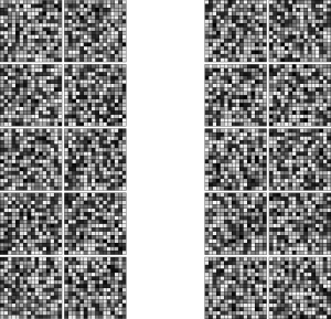
The Islanders have a shorter genome than regular humans and so make a manageable example to illustrate the principles of microarray analysis. Chloe Moore from Colmar University was interested in identifying any Islander genes related to the risk of diabetes. She recruited 20 subjects for her study, 10 without diabetes and 10 with diabetes. For each subject she conducted a microarray experiment. The figure below shows the resulting expression levels for each of the 10 subjects with diabetes and for each of the 10 subjects without diabetes. The question is whether there is any systematic difference between the intensity levels expressed in each set of images.
The figure below shows a more quantitative summary of the results with side-by-side box plots for each of the 256 genes appearing in the microarrays. For clarity we have indicated the median location with a horizontal line, rather than the dot we normally use. Look around the box plots and see if you can identify any genes where there may be a significant difference between the expression levels. (We will label the genes starting with B000 at the top left, going across to B015 at the top right and then proceeding down the plot to B255 in the bottom right.)

For each of the 256 genes we can carry out a two-sample [latex]t[/latex] test to compare the levels between the subjects with diabetes and those without. Each test gives a [latex]P[/latex]-value and these can be visualised with a Manhattan plot, seen below. In this plot the horizontal axis gives the gene position while the vertical axis gives the value [latex]-\log_{10}(p)[/latex] for each [latex]P[/latex]-value, [latex]p[/latex]. This transformation means that smaller [latex]P[/latex]-values will appear higher on the scale. For example, the highest value of around 3.0 corresponds to a [latex]P[/latex]-value of around [latex]10^{-3.0} = 0.001[/latex].

Four genes with strongest [asciimath]P[/asciimath]-values
| Gene | [asciimath]p[/asciimath] |
|---|---|
| B116 | 0.000998 |
| B041 | 0.001415 |
| B186 | 0.001559 |
| B118 | 0.005669 |
The table above shows the genes with the four strongest [latex]P[/latex]-values in terms of the difference in mean expression levels between the two groups and the following figure shows the corresponding box plots in more detail. The strongest of these, B116, has a very small [latex]P[/latex]-value of 0.000998. As an individual result we would take this to be substantial evidence that the expression of this gene was related to diabetes, with diabetic subjects having lower levels of expression than non-diabetic subjects. However, we have carried out 256 hypothesis tests — would we expect to find a [latex]P[/latex]-value this small by chance?

In our discussion of the Bonferroni correction above we were taking a fixed error rate and adjusting it to find the new error rate we should use in our analysis. Rather than compare [latex]P[/latex]-values to an adjusted [latex]\alpha[/latex] value, an alternative is to adjust the [latex]P[/latex]-values themselves (Wright, 1992). Here instead of dividing a target [latex]\alpha[/latex] by the number of tests, [latex]k = 256[/latex], we multiply the individual [latex]P[/latex]-values by 256 to obtain the adjusted P-value. The table below gives the results of this simple calculation and we see that the evidence is now much weaker. In particular, evidence for a B116 effect is now inconclusive.
Four genes with strongest adjusted [asciimath]P[/asciimath]-values
| Gene | [asciimath]p[/asciimath] (adjusted) |
|---|---|
| B116 | 0.255 |
| B041 | 0.362 |
| B186 | 0.399 |
| B118 | 1.000 |
Of course this adjustment is very conservative. All but three of the genes had [latex]P[/latex]-values that when multiplied by 256 gave probabilities above 1 (and so have been capped at 1). Wright (1992) discusses more sophisticated adjustments to multiple [latex]P[/latex]-values that you will find available in statistical software though the basic principle of correcting for a family-wise error rate is still the same. Reiner et al. (2003) gives an overview of alternative methods based on adjusting for the false discovery rate, the expected probability of false positives when looking for factors affecting gene expression.
Note that even though the results of this microarray study have been inconclusive they do help direct further research. B116 and the other strongest genes can be taken as candidates for more detailed investigation.
Tukey’s Honestly Significant Difference
The problem with making conclusions from a posteriori comparisons, those that we think of only after looking at the data, is that we will look for the largest difference between sample means. With lots of pairwise comparisons it can be quite likely this largest difference is significant even if all the population means were the same. The Bonferroni correction is a simple way of dealing with this, reducing the individual error rate to compensate. A more sophisticated approach is given by Tukey (1953).
The idea behind Tukey’s method is to actually use the sampling distribution of the largest standardised difference found when comparing [latex]k[/latex] groups which all have the same means and standard deviations. This distribution is called the Studentised range distribution, [latex]Q(k,d)[/latex], where [latex]k[/latex] is the number of groups and [latex]d[/latex] is the residual degrees of freedom. The method described here is only valid for the case of equal replications in each group. Steel and Torrie (1960) give modifications for the more general case.
The Tukey statistic is a minor modification of the regular [latex]t[/latex] statistic with
\[ q_{k,d} = \frac{|\overline{x}_i – \overline{x}_j|}{\sqrt{\frac{\mbox{MSR}}{n}}}, \]
where [latex]n[/latex] is the number of replications in each group. For example, for comparing treatments [latex]C[/latex] and [latex]F[/latex] in the potato experiment we would have
\[ q_{6,30} = \frac{124}{60.33/\sqrt{6}} = 5.03. \]
Instead of comparing to the [latex]t[/latex] distribution, we obtain bounds on the [latex]P[/latex]-value from the critical values of the Studentised range distribution at the end of this chapter. Here we find that the [latex]P[/latex]-value is between 0.05 and 0.01, some evidence of a difference between [latex]C[/latex] and [latex]F[/latex] in their mean potato yield.
As with the two-sample [latex]t[/latex] test, the denominator of this statistic is the same for each pairwise comparison and so we can determine the minimum difference that would be significant. The critical value for 5% significance from the Studentised range distribution is [latex]q_{6,30}^{*} = 4.30[/latex] so that the difference must be at least
\[ 4.30 \times \frac{60.33}{\sqrt{6}} = 105.9 \mbox{ lbs}. \]
This value is known as Tukey’s Honestly Significant Difference (HSD). Note that is it higher than the least significant difference, 71.1 lbs, found earlier in this chapter, taking into account the multiple comparisons by requiring a higher threshold for significance. However it is less conservative than the Bonferroni correction where the corresponding value was 111.1 lbs.
You can refer back to the list of pairwise differences in the earlier table and compare each one to the HSD to assess significance. Alternatively, the table below used software to calculate the [latex]P[/latex]-values from the Studentised range distribution for each pairwise difference.
Pairwise Tukey tests for differences in mean yield (lbs)
| Pair | [asciimath]q_{6,30}[/asciimath] | [asciimath]P[/asciimath]-value |
|---|---|---|
| A - B | 3.31 | 0.210 |
| A - C | 5.39 | 0.008 |
| A - D | 2.44 | 0.525 |
| A - E | 7.11 | <0.001 |
| A - F | 10.43 | <0.001 |
| B - C | 2.08 | 0.683 |
| B - D | 0.87 | 0.989 |
| B - E | 3.80 | 0.107 |
| B - F | 7.12 | <0.001 |
| C - D | 2.95 | 0.321 |
| C - E | 1.72 | 0.826 |
| C - F | 5.03 | 0.014 |
| D - E | 4.67 | 0.027 |
| D - F | 7.98 | <0.001 |
| E - F | 3.32 | 0.208 |
Note that if we were just comparing two groups then the critical value would be [latex]q_{2,30}^{*} = 2.89[/latex] and so the HSD would be
\[ 2.89 \times \frac{60.33}{\sqrt{6}} = 71.1 \mbox{ lbs}. \]
This is just the LSD, again illustrating that Tukey’s HSD is taking into account the multiple comparisons being performed by increasing the threshold for significance.
The advantage of the LSD and Bonferroni methods is that they can be performed using standard [latex]t[/latex] procedures. The Bonferroni method may also be preferable if there is a valid a priori limit on the number of comparisons being made. However, in software the Tukey procedure is often the standard approach available.
Summary
- The least significant difference can be used to quickly make pairwise comparisons.
- Making multiple comparisons leads to an inflation of the family error rate which needs to be corrected.
- The Bonferroni correction adjusts the individual error rate to satisfy a target family error rate, such as 5%.
- The Tukey correction uses the distribution of the largest difference to adjust the width of intervals based on the number of comparisons being made.
Exercise 1
Three paper planes were made using plain A3 and A4 sized paper that was cut to size to achieve chosen wingspan values. The same model and type of paper were used to make each plane. Each paper plane was tested for ten successful fights over a clear course. The distances flown are given in the table below.
Distance flown (cm) with different wingspans (cm)
| Wingspan | Distance | |||||||||
|---|---|---|---|---|---|---|---|---|---|---|
| 6 | 150 | 167 | 167 | 220 | 241 | 245 | 283 | 307 | 310 | 368 |
| 4 | 195 | 275 | 300 | 311 | 230 | 271 | 175 | 302 | 281 | 225 |
| 2 | 293 | 289 | 296 | 301 | 324 | 300 | 340 | 294 | 288 | 269 |
Carry out a one-way analysis of variance to determine whether the mean distance flown by paper planes differs between the three wingspan groups. Calculate the three possible confidence intervals between means, using appropriate corrections.
Exercise 2
The previous question could also be carried out using regression, with wingspan as a quantitative predictor variable. Compare the results and interpretations between these two approaches. Which seems most appropriate for this data?
Exercise 3
Use the HSD value from the potato yield example to assess the significance of the differences in the table of pairwise differences. Compare your results with the [latex]P[/latex]-values given in the table of pairwise Tukey tests.
Exercise 4
Calculate the LSD and HSD values for the wind speed and water loss example in Chapter 19. Use each of these to determine which differences might be significant and compare your results.
Studentized Range distribution [latex]Q(k,d)[/latex]
| [latex]d[/latex] | [latex]p[/latex] | [latex]k=[/latex]2 | 3 | 4 | 5 | 6 | 7 | 8 | 9 | 10 |
|---|---|---|---|---|---|---|---|---|---|---|
| 1 | 0.05 | 18.0 | 27.0 | 32.8 | 37.1 | 40.4 | 43.1 | 45.4 | 47.4 | 49.1 |
| 0.01 | 90.0 | 135 | 164 | 186 | 202 | 216 | 227 | 237 | 246 | |
| 2 | 0.05 | 6.08 | 8.33 | 9.80 | 10.9 | 11.7 | 12.4 | 13.0 | 13.5 | 14.0 |
| 0.01 | 14.0 | 19.0 | 22.3 | 24.7 | 26.6 | 28.2 | 29.5 | 30.7 | 31.7 | |
| 3 | 0.05 | 4.50 | 5.91 | 6.82 | 7.50 | 8.04 | 8.48 | 8.85 | 9.18 | 9.46 |
| 0.01 | 8.26 | 10.6 | 12.2 | 13.3 | 14.2 | 15.0 | 15.6 | 16.2 | 16.7 | |
| 4 | 0.05 | 3.93 | 5.04 | 5.76 | 6.29 | 6.71 | 7.05 | 7.35 | 7.60 | 7.83 |
| 0.01 | 6.51 | 8.12 | 9.17 | 9.96 | 10.6 | 11.1 | 11.5 | 11.9 | 12.3 | |
| 5 | 0.05 | 3.64 | 4.60 | 5.22 | 5.67 | 6.03 | 6.33 | 6.58 | 6.80 | 6.99 |
| 0.01 | 5.70 | 6.98 | 7.80 | 8.42 | 8.91 | 9.32 | 9.67 | 9.97 | 10.2 | |
| 6 | 0.05 | 3.46 | 4.34 | 4.90 | 5.30 | 5.63 | 5.90 | 6.12 | 6.32 | 6.49 |
| 0.01 | 5.24 | 6.33 | 7.03 | 7.56 | 7.97 | 8.32 | 8.61 | 8.87 | 9.10 | |
| 7 | 0.05 | 3.34 | 4.16 | 4.68 | 5.06 | 5.36 | 5.61 | 5.82 | 6.00 | 6.16 |
| 0.01 | 4.95 | 5.92 | 6.54 | 7.00 | 7.37 | 7.68 | 7.94 | 8.17 | 8.37 | |
| 8 | 0.05 | 3.26 | 4.04 | 4.53 | 4.89 | 5.17 | 5.40 | 5.60 | 5.77 | 5.92 |
| 0.01 | 4.75 | 5.64 | 6.20 | 6.62 | 6.96 | 7.24 | 7.47 | 7.68 | 7.86 | |
| 9 | 0.05 | 3.20 | 3.95 | 4.41 | 4.76 | 5.02 | 5.24 | 5.43 | 5.59 | 5.74 |
| 0.01 | 4.60 | 5.43 | 5.96 | 6.35 | 6.66 | 6.91 | 7.13 | 7.33 | 7.49 | |
| 10 | 0.05 | 3.15 | 3.88 | 4.33 | 4.65 | 4.91 | 5.12 | 5.30 | 5.46 | 5.60 |
| 0.01 | 4.48 | 5.27 | 5.77 | 6.14 | 6.43 | 6.67 | 6.87 | 7.05 | 7.21 | |
| 11 | 0.05 | 3.11 | 3.82 | 4.26 | 4.57 | 4.82 | 5.03 | 5.20 | 5.35 | 5.49 |
| 0.01 | 4.39 | 5.15 | 5.62 | 5.97 | 6.25 | 6.48 | 6.67 | 6.84 | 6.99 | |
| 12 | 0.05 | 3.08 | 3.77 | 4.20 | 4.51 | 4.75 | 4.95 | 5.12 | 5.27 | 5.39 |
| 0.01 | 4.32 | 5.05 | 5.50 | 5.84 | 6.10 | 6.32 | 6.51 | 6.67 | 6.81 | |
| 13 | 0.05 | 3.06 | 3.73 | 4.15 | 4.45 | 4.69 | 4.88 | 5.05 | 5.19 | 5.32 |
| 0.01 | 4.26 | 4.96 | 5.40 | 5.73 | 5.98 | 6.19 | 6.37 | 6.53 | 6.67 | |
| 14 | 0.05 | 3.03 | 3.70 | 4.11 | 4.41 | 4.64 | 4.83 | 4.99 | 5.13 | 5.25 |
| 0.01 | 4.21 | 4.89 | 5.32 | 5.63 | 5.88 | 6.08 | 6.26 | 6.41 | 6.54 | |
| 15 | 0.05 | 3.01 | 3.67 | 4.08 | 4.37 | 4.59 | 4.78 | 4.94 | 5.08 | 5.20 |
| 0.01 | 4.17 | 4.84 | 5.25 | 5.56 | 5.80 | 5.99 | 6.16 | 6.31 | 6.44 | |
| 16 | 0.05 | 3.00 | 3.65 | 4.05 | 4.33 | 4.56 | 4.74 | 4.90 | 5.03 | 5.15 |
| 0.01 | 4.13 | 4.79 | 5.19 | 5.49 | 5.72 | 5.92 | 6.08 | 6.22 | 6.35 | |
| 17 | 0.05 | 2.98 | 3.63 | 4.02 | 4.30 | 4.52 | 4.70 | 4.86 | 4.99 | 5.11 |
| 0.01 | 4.10 | 4.74 | 5.14 | 5.43 | 5.66 | 5.85 | 6.01 | 6.15 | 6.27 | |
| 18 | 0.05 | 2.97 | 3.61 | 4.00 | 4.28 | 4.49 | 4.67 | 4.82 | 4.96 | 5.07 |
| 0.01 | 4.07 | 4.70 | 5.09 | 5.38 | 5.60 | 5.79 | 5.94 | 6.08 | 6.20 | |
| 19 | 0.05 | 2.96 | 3.59 | 3.98 | 4.25 | 4.47 | 4.65 | 4.79 | 4.92 | 5.04 |
| 0.01 | 4.05 | 4.67 | 5.05 | 5.33 | 5.55 | 5.73 | 5.89 | 6.02 | 6.14 | |
| 20 | 0.05 | 2.95 | 3.58 | 3.96 | 4.23 | 4.45 | 4.62 | 4.77 | 4.90 | 5.01 |
| 0.01 | 4.02 | 4.64 | 5.02 | 5.29 | 5.51 | 5.69 | 5.84 | 5.97 | 6.09 | |
| 21 | 0.05 | 2.94 | 3.56 | 3.94 | 4.21 | 4.42 | 4.60 | 4.74 | 4.87 | 4.98 |
| 0.01 | 4.00 | 4.61 | 4.99 | 5.26 | 5.47 | 5.65 | 5.79 | 5.92 | 6.04 | |
| 22 | 0.05 | 2.93 | 3.55 | 3.93 | 4.20 | 4.41 | 4.58 | 4.72 | 4.85 | 4.96 |
| 0.01 | 3.99 | 4.59 | 4.96 | 5.22 | 5.43 | 5.61 | 5.75 | 5.88 | 5.99 | |
| 23 | 0.05 | 2.93 | 3.54 | 3.91 | 4.18 | 4.39 | 4.56 | 4.70 | 4.83 | 4.94 |
| 0.01 | 3.97 | 4.57 | 4.93 | 5.20 | 5.40 | 5.57 | 5.72 | 5.84 | 5.95 | |
| 24 | 0.05 | 2.92 | 3.53 | 3.90 | 4.17 | 4.37 | 4.54 | 4.68 | 4.81 | 4.92 |
| 0.01 | 3.96 | 4.55 | 4.91 | 5.17 | 5.37 | 5.54 | 5.69 | 5.81 | 5.92 | |
| 25 | 0.05 | 2.91 | 3.52 | 3.89 | 4.15 | 4.36 | 4.53 | 4.67 | 4.79 | 4.90 |
| 0.01 | 3.94 | 4.53 | 4.89 | 5.14 | 5.35 | 5.51 | 5.65 | 5.78 | 5.89 | |
| 26 | 0.05 | 2.91 | 3.51 | 3.88 | 4.14 | 4.35 | 4.51 | 4.65 | 4.77 | 4.88 |
| 0.01 | 3.93 | 4.51 | 4.87 | 5.12 | 5.32 | 5.49 | 5.63 | 5.75 | 5.86 | |
| 27 | 0.05 | 2.90 | 3.51 | 3.87 | 4.13 | 4.33 | 4.50 | 4.64 | 4.76 | 4.86 |
| 0.01 | 3.92 | 4.49 | 4.85 | 5.10 | 5.30 | 5.46 | 5.60 | 5.72 | 5.83 | |
| 28 | 0.05 | 2.90 | 3.50 | 3.86 | 4.12 | 4.32 | 4.49 | 4.62 | 4.74 | 4.85 |
| 0.01 | 3.91 | 4.48 | 4.83 | 5.08 | 5.28 | 5.44 | 5.58 | 5.70 | 5.80 | |
| 29 | 0.05 | 2.89 | 3.49 | 3.85 | 4.11 | 4.31 | 4.47 | 4.61 | 4.73 | 4.84 |
| 0.01 | 3.90 | 4.47 | 4.81 | 5.06 | 5.26 | 5.42 | 5.56 | 5.67 | 5.78 | |
| 30 | 0.05 | 2.89 | 3.49 | 3.85 | 4.10 | 4.30 | 4.46 | 4.60 | 4.72 | 4.82 |
| 0.01 | 3.89 | 4.45 | 4.80 | 5.05 | 5.24 | 5.40 | 5.54 | 5.65 | 5.76 | |
| [latex]\infty[/latex] | 0.05 | 2.77 | 3.31 | 3.63 | 3.86 | 4.03 | 4.17 | 4.29 | 4.39 | 4.47 |
| 0.01 | 3.64 | 4.12 | 4.40 | 4.60 | 4.76 | 4.88 | 4.99 | 5.08 | 5.16 |
This table gives gives [latex]q^{*}[/latex] such that [latex]\pr{Q_{k,d} \ge q^{*}} = p[/latex].
