
Chapter 12: Non-Market Valuation Methods
Learning Objectives
After completing this chapter, students should be able to:
-
Define total economic value.
-
Identify types of goods including public goods, common goods, and mixed goods.
-
Value impacts using alternative market pricing methods.
-
Compare and contrast revealed and stated preference approaches to non-market valuation.
-
Implement and evaluate non-market valuations.
Introduction
Continuing with the valuation of benefits and costs, we come to the final key concept – non-market valuation. It has been assumed that all impacts of policies and programs can be measured using market prices, or when markets are distorted, it is possible to adjust the observed market prices to reflect the true economic value of a good or service. However, this is not possible in all cases of market failure. Specifically, this chapter focuses on how to value goods and services when the appropriate market is absent. i.e., goods and services that are not traded on markets or cannot be traded on markets resulting in no observed market price.
In this chapter, we will explore methods for ascertaining the economic value of a good or service in situations where a market price is not available. The approaches discussed are particularly useful for policy or projects with social, health, or environmental aspects. In particular, non-market valuation methods are useful for evaluating intangible impacts, such as national pride, climate abatement, pollution costs, public goods, and common goods. Consequently, non-market valuations are more common in public sector CBA, where the government is evaluating a policy or project. Specifically, the government is often interested in projects that may have wider intangible impacts or the resource is not provided by the private sector.
To being our approach to non-market valuations, we first need to understand the concept of total economic value.
Total Economic Value
Value and price are two different concepts in cost-benefit analysis. The price is the amount economic agents are willing to pay for a good or service on a market. The economic value is the benefit derived from the good or service. In the absence of market distortions and market failures, the economic value and the price would be equivalent. However, economic value and price are often not equivalent if we observe market failure, market distortions, or market absence. For example, many environmental goods are not traded on markets and therefore there is no market price that can reveal the willingness-to-pay to consume the environmental good or service. Hence, we often refer to the total economic value in cost-benefit analysis, which aggregates all benefits from the use of a resource.
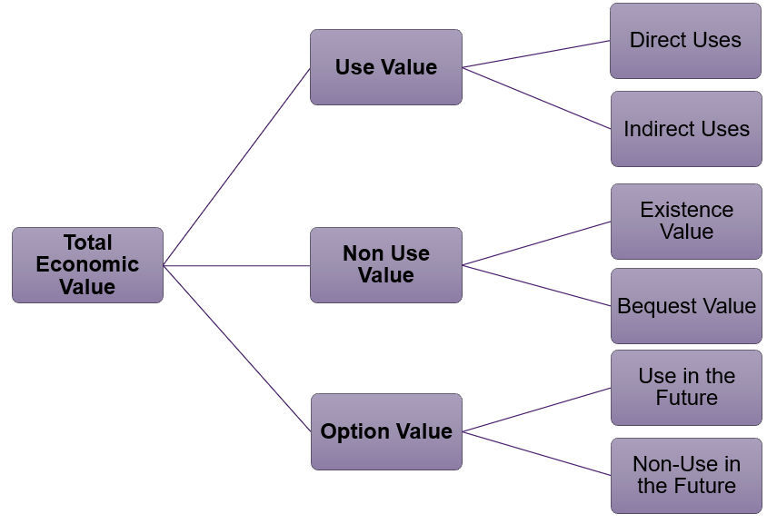
Total economic value is a concept that is key to cost-benefit analysis. Total economic value refers the value derived from a resource (such as the environment). The total economic value captures the overall economic value of the resource to society. There are three components to total economic value highlighted in equation (1).
(1) 
Use value consists of direct use value and indirect use value. Direct use value can be from consumptive uses and non-consumptive uses.[1] For example, if we consider a national park consumptive uses may include catching fish for food or using trees as wood for fires. Non-consumptive uses include hiking and birdwatching. Non-consumptive uses do not diminish the availability of the resources for others, whereas consumptive uses diminish the availability of the resource in the future. In these instances, an economic agent is deriving utility from direct use of the resource capturing recreation values.
Indirect use values are the benefits derived from the resource without actually “using” the resource directly or being near the resource. Coming back to the example of the national park this would include climate regulation, air and water purification, biodiversity benefits, etc. Estimating indirect uses is one of the biggest challenges faced by CBA analysts.
Non-use value captures existence value and bequest value. Existence value is the value attained by economic agents by knowing that a resource is conserved and will continue to exist. Within the national park example, this would be the knowledge that the parkland and its wildlife is protected even if you never visit the location. This is especially relevant for threatened or endangered species of flora and fauna. Similarly, bequest value is value gained from preserving the resource to be passed onto future generations, even if those future generations choose not to utilise the resource itself.
Option value reflects the value placed on the ability to use the resource in the future. The option value should capture the potential future benefits from the resource. Similar to use values – option value can subsequently be separated into direct and indirect uses.
The components of total economic value are illustrated in Figure 12.1 below:
Obviously, when apply shadow pricing to non-market goods and services, it is much more challenging than adjusting the observed market prices as seen in Chapter 8. It is crucial to capture all aspects of the total economic value in the approach to shadow pricing.
Total economic value has implications for CBA. Categorically speaking, the implications relate to identifying the appropriate shadow price to be used in the social CBA. When dealing with non-market goods and services the value of the good is not reflected in market prices. The approach to the non-market value for a particular good or service under evaluation requires consideration of the role of use, non-use, and option values for the underlying resource. This represents a challenge for CBA analysts. Consequently, the type of non-market valuation methodology will relate directly to the aspect of total economic value we choose to identify and estimate, which is also dependent on the type of good the resource can be categorised as.
Types of Goods
When approaching non-market evaluation, it is important for the analyst to think of any resource or commodity as lying on a continuum between a pure public good and a pure private good. Usually, economists define goods based on their level of excludability and rivalrousness in consumption:
- Excludability: If an individual can be prevented from consuming a good or service, it is considered excludable.
- Rivalrous: If an individual’s consumption of a good diminishes the availability of the good for others to consume, then it is considered rivalrous.
All goods can lie on the continuum between pure private goods and pure public goods. However, for simplicity, we identify four key categories for goods outlined in Figure 12.2: (1) private goods, (2) club goods, (3) common goods, and (4) public goods.
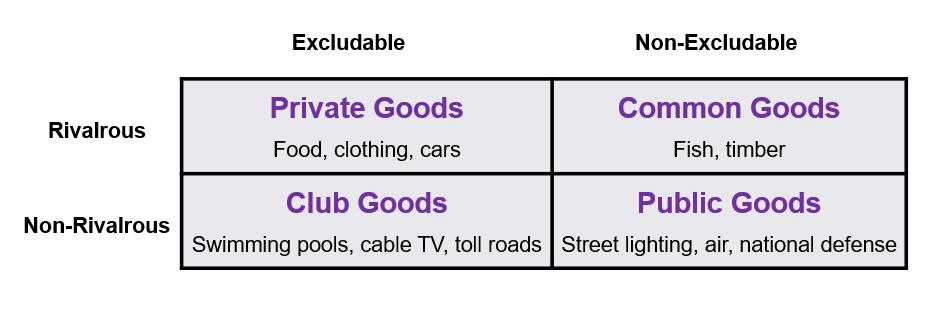
– Private goods – are excludable and rivalrous. For example, mobile devices and laptops. These are purchased in stores (excludable) and when you purchase the device the quantity on the market decreases (rivalrous).
– Club goods – also known as mixed goods, are excludable but non-rival. For example, toll roads are excludable via the use of a paid toll, but are non-rival as your use of the toll road does not decrease the availability of the road to other users who have also paid the toll.
– Common goods – are non-excludable, but rivalrous. For example, the fish stock in the Pacific ocean is a common good. Everyone can fish from the Pacific ocean (non-excludable). However, as the fish stock is taken from the ocean the number of fish available decrease, depleting the stock of fish over time (rivalrous). Common goods are often affected by the tragedy of the commons.
– Public goods – are non-excludable and non-rival. A good example of public goods is street lighting. You cannot be excluded from using a streetlight (non-excludable) and when using the streetlight, you do not diminish the availability of the light for other users of the light (non-rivalrous). Public goods are subject to free-rider problems.
As non-market goods and services are those not bought or sold directly on markets and therefore do not have an associated market price, they tend to fall into the categories of public goods or common goods. For example, common goods include beaches and national parks. Public goods include clean air and street lighting.
To capture the true net social benefit in a policy or project, it is therefore essential for an analyst to capture the impacts of common and public goods as part of their analysis.
Non-Market Goods and Services in CBA
When goods and services have no market, we still need to evaluate the impact of these goods and services as part of the evaluation of a policy or project. Consequently, shadow prices are used for valuing goods and services not actively traded on markets. For example, we often estimate shadow prices for:
- Externalities
- Public Goods
- Common Goods
Ideally, when implementing non-market valuation into CBA we are attempting to value benefits such as nature, recreation, water quality, climate abatement, prevention of disease, value of life, etc. When dealing with non-market costs we are trying to value air pollution, noise pollution, light pollution, environmental degradation, overfishing, etc. Inherently, these non-market benefits and costs are difficult to measure. By their nature there is no direct market for determining their economic value of these goods and services, and thus the appropriate shadow price is hard to determine.
To ensure social surplus is maximised effectively, governments see a need to regulate the private market or undertake public expenditure in areas that are neglected by the market. The government tends to be the supplier of public goods, as the private sector has no incentive to produce the good or service. The result is that the government therefore needs to know which goods to provide as public goods to maximise the use of public sector resources and hence non-market valuation is necessary.
Challenges of Non-Market Valuation
Non-market goods and services are also important for cost-benefit analysis. Even though non-market goods and services are not traded on markets, evaluating them as part of a CBA is crucial to calculating the total economic welfare. So even though we do not know the price, we still need to take into account the economic value of non-market goods and services.
If non-market goods and services are excluded from a social CBA, it introduces omission bias into the estimation of the net social benefit. It is crucial to note, that the investor CBA perspective would ignore the role of non-market impacts.
Consequently, an analyst is likely to encounter non-market valuation challenges. If project inputs and project outputs are not fully accounted for in a social CBA, it is not possible to reach allocative efficiency.
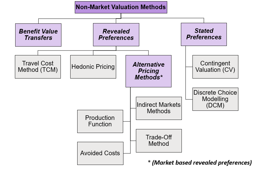
Approaches to Non-Market Methods
There are many ways to approach non-market valuation as highlighted in Figure 12.3. As mentioned in Chapter 7, benefit value transfers are a good starting point for evaluation of non-market benefits and costs.
Benefit Transfer Methods
Most non-market valuation methods are technically complex, costly, and time consuming to implement. In the context of most CBA preparations, it is usually not be feasible for an individual department to undertake its own non-market valuation study for an individual project or policy. However, this does not necessarily mean we cannot attach a monetary value to the relevant non-market costs or benefits. Numerous non-market valuation studies have been compiled around many parts of the world. This means that it is possible to ‘borrow’ an approximate value (or a range of values) from other studies in similar situations – known as benefit value transfers.
Drawing directly on benefit transfers discussed in Chapter 7, there is extensive research on non-market valuations for common externalities and public goods. Prices such as the social cost of carbon, tobacco externalities etc, have utilised non-market valuation methods to calculate the impact or economic value used in analysis. Meta analysis often highlights specific methodological approaches. It is possible to utilise benefit transfers from existing research – however if we want to adjust or improve these plug-in values it is necessary to understand how to implement non-market valuation methods. To evaluate the existing literature for utilisation for a project currently under consideration, it is important for an analyst to understand the methodological approaches to non-market valuations, including their advantages and disadvantages.
Alternative Pricing Methods
Alternative pricing methods for non-market valuation using involves find alternative pricing mechanisms from already available information. There are four key alternative pricing approaches; indirect markets, opportunity costs, avoided costs, and production.
Indirect Markets (Market Analogy Method)
This method is often used by the government sector to determine how much of a good or service the government needs to supply. Examples of this method include education, public housing, and healthcare. To implement the indirect market method, we begin by finding similar goods and services in a private market. The good or service must be comparable to the public good or service we are trying to value as part of the public project. Once an appropriate market is identified, we can use the information on the private market to estimate the value of the good or service if it was provided publicly by the government. Specifically, we can utilise the information on willingness-to-pay in the private market to identify what the price and quantity would be in the public market. The data from the private market is then used as a surrogate for the publicly provided good if their markets are similar. After analysing the similar market, it can be determined if the market price of a comparable good in the private sector can be an appropriate shadow price for the good used in the public sector.
Example 12.1
Example – Indirect Market for Public Housing
Suppose the government wishes to provide some public housing. In this instance the government is providing rental housing lower than the market price. Suppose we observe the following information on the rent in the two markets:
Public Housing Rent: $1,750 per month
Private Housing Rent: $2,500 per month
Those who require public housing are not likely to value the housing at $2,500 per month, but they will value it above $1,750 per month. Therefore the willingness-to-pay for the public housing will lie between $1,750 and $2,500 per month. This information can then subsequently be used to determine how the government should value public housing when considering similar projects.
Disadvantage of this approach include:
- Requires the tastes, preferences, and quality to be the same between the consumers of the public good and the private good.
- Using private sector revenues would also often underestimate the benefits as it ignores the consumer surplus.
Trade-off Method (Opportunity Costs)
We already know that CBA analysts can use opportunity costs to evaluate a policy or project. Opportunity costs can also be used to evaluate non-market impacts. In the past we have looked at how to value time saved and the value of statistical life using wages. For example, we can use labour market wages to value time saved from reduced traffic congestion for road construction projects.
Disadvantage of this approach include:
- Using wages ignores other potential benefits and is subject to market failures. For example, some people may be unable to change their working hours each week, or firms may not be paying their employees their marginal social product.
- Using after tax wages may not effectively capture the true opportunity cost as it ignores individual preferences and the role of before-tax earnings on decision-making (Whittington & Cook, 2019).
- Using after tax wages ignores benefits from the project related to and the impact of taxes on preferences.
- It ignores potential for multitasking – for example people could be working while waiting or travelling resulting in the CBA underestimating the effects.
- Makes the assumption that people value the many uses of their time the same. However, the value of time saved travelling, time at work, and time spent in leisure activities are often valued differently based on personal preferences.
Consequently, there are quite a few disadvantages of this method when using wages as the opportunity cost. Analysts usually cannot know for sure how trade-offs are made and whether using wages would capture the full opportunity cost involved.
Example 12.2
Trade-Off Method – Value of Statistical Life
Government health and safety programs often need to obtain a monetary value for lives saved after implementing a policy or program. This is referred to as the value of statistical life (VSL).[2]
It is possible to use the trade-off method to calculate a VSL in three ways:
1) Foregone Earnings Method – the lives saved is equal to the person’s discounted future earnings. This method is often used in compensation cases within the legal context. There are ethical and moral limitation of this method that have led to a general consensus that this method is inappropriate. The foregone earnings method provides of higher values for higher income earners and lower values for low-income earners (discriminating between professions). There are also elements of gender biases as women often self-select into lower income professions. Furthermore, for retired people the result of VSL may be negative. This is problematic if we consider healthcare interventions where older people need more interventions, but the value attached to their statistical lives is lower.
2) Simple Consumer Purchases – willingness-to-pay for a reduction in risk. Specifically, we evaluate the purchase of safety equipment or other life-saving devices to reduce the risk of death. If people are indifferent between paying an extra $300 to reduce the probability of death by 1/10,000 – then their life is valued at $3 million (price paid / risk reduction = $300 / (1/10,000)). This is a revealed preference.
3) Simple Labour Market Studies – comparing the risk premium for taking a risky job over a less risky job. If a person is willing to forgo an extra $3,500 per year to increase the probability, they will not have a fatal accident at work by 1/1,000 – then the person values their live at $3.5 million or more (forgone earnings/ risk reduction = $3,500/(1/1,000). This is also a revealed preference.
Avoided Costs (Mitigating Behaviours)
People can place a price on a non-market impact through the process of paying to avoid or mitigate the impact. For example, climate abatement costs, or double glazing windows to reduce noise pollution. The transactions associated with avoided costs can be used as a proxy value in the CBA.
Disadvantage of this approach include:
- The avoided cost method has been criticised for using price to proxy for economic surpluses, and consequently underestimating the true value of the non-market good or service (Baker and Ruting, 2014).
Production Function
Production function methods involves modelling consumer behaviour. The production function approach involves investigating changes in the availability or consumption of goods and services that are substitutes or compliments of the non-market good or service of interest. For environmental goods and services, the contribution to the final market production is captured.
Case Study – Beekeeping and Production Function
If we go back to the example of beekeeping as a positive externality from Chapter 8. It is possible to use the production function method to value the benefit of the effects of bees as pollinators and pollination services on total crop output, capturing relative benefits to other goods and services outside of honey production. This method when applied to the benefits of pollination is considered highly accurate (Gallai, 2016).
Disadvantage of this approach include:
- One off the issues with using the production function method is the requirement for full information regarding the contribution to production. As there is incomplete scientific understanding of the environmental impacts or changes it can create bias in the estimates (Baker and Ruting, 2014).
Alternative Market Pricing Overall
There are some common advantages and disadvantages of using alternative market pricing approaches to non-market valuation.
- Advantage: Provides a non-zero valuation of the non-market good or service which would otherwise not be included in a CBA. It’s better to have included an impact as a non-zero value than excluded it from the CBA by setting the value equal to zero.
- Disadvantage: Issues with omitted variable biases. Using alternative market approaches may not capture the non-use value or option value of a good or service, leading to omitted variable bias.
- Disadvantage: There is opportunity to introduce selection bias based on the approach used. For example, if we use an inappropriate market for the indirect market method.
Furthermore, all the alternative pricing methods relied on indirect approaches to pricing. Consequently, these methods are examples of revealed preferences – meaning that individual’s preferences are revealed by their interaction on the market.
Stated Preferences Versus Revealed Preferences
When using non-price related methods to value non-market benefits and costs, we often rely on revealed or stated preference approaches for valuation. A preference is the order that a person gives to alternatives based on their relative utility. By ranking their preferences an individual can make the optimal choice that maximises their utility. Expanding on this, revealed preferences are preferences revealed by studying actual decisions people make (measured by their actions) to determine the value of non-market goods and services. Stated preferences approaches to non-market valuation are survey-based approaches to valuation. For stated preferences, individuals are asked about their willingness-to-pay or willingness-to-accept under a series of hypothetical decisions.
Revealed Preference Methods
Revealed preferences are founded in actual behaviours that can be observed and provide a reliable estimate of non-market valuations. However, non-use value is often not reflected in the observed behaviours in the market. Therefore, revealed preference methods best for evaluating non-market impacts that are heavily weighted towards use values.
There are two key revealed preference methods that are used to study the actual decisions people make regarding the non-market goods and services; (1) hedonic pricing, and (2) travel cost method.
Hedonic Pricing Method
The hedonic pricing method assumes that the value of non-market goods and services is partially reflected in the price paid for an underlying asset, item, good, or service. By deconstructing the price of a multiple attribute market good, hedonic pricing can capture the price of non-market attribute or aspect of the good. Systematic variation in the price of the underlying asset allows the analyst to capture the value of the non-market characteristic or resource under evaluation. This allows for an implicit price for each attribute the consumer is willing to pay including those attributes that are not traded on markets. For example, we can use hedonic pricing to capture the non-market value of noise pollution, proximity to beaches, or recreational facilities through the price paid for housing.
To estimate a hedonic pricing model, an analyst identifies a function with price as the dependent variable and the attributes of the good as independent variables, including the non-market attribute in question. For example, if we were interested in how the view impacts the price of a house, we may choose to estimate the following multiplicative model:

where SIZE is the size of the land the house is on, BEDS is the number of bedrooms, VIEW is the view of the house (the non-market attribute we wish to value) and QUALITY is the quality of the building. This function would be referred to as the hedonic price function or implicit price function. Converting this multiplicative model into logarithms and regressing the results will give the elasticities i.e., the coefficient on VIEW ( ) would tell us the WTP for an average house in response to a 1% increase in the “quality of the view” – the non-market attribute. Consequently, we can observe the change in the price of a house that results from a unit change in a particular attribute (i.e., the slope). This is called the hedonic price, implicit price, or rent differential of the attribute.
After identifying the hedonic price, the second step to evaluating the non-market attribute is to use the estimates for the WTP to derive the demand for the specific attribute in question. When implementing the second step, we should control for preferences which can be captured by factors such as income and other socioeconomic variables. For example, we could estimate the following:

where INC is the household income, SOCEC is a vector of socioeconomic characteristics (such as age, gender, postcode, etc.). Once formulated, we can use the results from the estimated demand curve to calculate any changes in consumer surplus as a result from a change in the non-market attribute of interest (in this case the view), by aggregating across all households.
There are two key advantages of the hedonic pricing method:
- The underlying application is conceptually intuitive and utilises prices that can be observed on a market.
- The results are based on revealed preferences which represent individual’s actual behaviours. Therefore, this method offers a way to overcome problems related to omitted variable bias and self-selection bias.
There are quite a few disadvantages of this method:
- The implication of the underlying non-market attribute being evaluated must be understood by the analyst. For example, people should know the amount of noise or the quality of the view when valuing these aspects using the hedonic pricing model.
- All inputs in the regression model must be measured without errors to ensure the analysis is sound and there are no multicollinearity issues.
- The functional form for the hedonic pricing function must be correctly specified.
- There should be a sufficient number of data points to ensure a sufficient number of comparison points i.e., all possible combinations of attributes are available to each individual purchasing on the market.
- The market price can adjust immediately to a change in the attributes that comprise the asset.
- It assumes that the value of the underlying asset can be calculated through the sum of the attributes alone.
Points 2, 3, and 4 are considered econometric problems with model specification.
Travel Cost Method
The travel cost method evaluates the expenses incurred travelling to make use of a good, service, or resource. The number of visits to a site is postulated to be a function of the travel cost and socioeconomic variables. The travel cost itself is a proxy for the price to use the good, service, or resource. The travel cost method is widely applied to recreational sites such as national parks, sporting fields, fishing, and tourism.
Suppose we wish to estimate the value of a national park. We expect that the number of visits demanded by an individual depends on the price ( ), the price of substitute activities (
 ), the individual’s income (
 ), and the preferences (
 ) of the individual such that we can estimate the following equation:

The price of the visit must capture the full price paid for a person to visit the local park. In this instance it is more than an admission fee or entry fee. It should include all opportunity costs involved including time spent travelling, any overnight accommodation, parking fees, etc. The sum of all the incurred expenses or costs to utilise the park count towards the total cost of the visit (the “price”). The total cost is then used in an explanatory variable to estimate the number of visits to the park – this measures the demand for the non-market good and service.
It is important to note that although the cost of admission into the facility being evaluated is usually the same, the total cost faced by each person varies. This allows for inference regarding the demand curve. Overall, using this method it is possible to estimate a demand curve for a good or service that does not have an underlying market. Once the demand curve is identified, we can apply the standard economic approaches to the evaluation of a CBA.
Estimating the demand schedule for a particular recreational site can be done in three east steps:
- Select a random sample of individuals or households within a defined boundary of the recreational site. These are the potential visitors.
- Survey the households to determine their number of visits over a period of time including the cost of the visits, the cost of visiting other recreational sites, their household’s income, and other characteristics that may affect their demand (such as the number of children in the household).
- Specify the functional form for the demand curve and estimate it using the data collected in step 2. Note that if the total cost replaces the price of the visit in the functional form, then quantity is a function of cost (and not the usual quantity as a function of price).
There are two key advantages of the travel cost method:
- The demand curve is relatively easy to estimate once the data is collected.
- Like the hedonic pricing method, the results are based on revealed preferences which represent individual’s actual behaviour. Therefore, this method offers a way to overcome problems related to omitted variable bias and self-selection bias.
The disadvantages of the travel cost method include:
- The estimates are the WTP for an entire site and not a specific feature of the site. For example, in evaluating the national park, you would estimate the value of the park for hiking, fishing, and camping all together. Therefore, you cannot identify a value for a specific non-market aspect of the site.
- Measuring total cost per visit is difficult as you also need to measure the opportunity cost. Opportunity costs need to be fully measured – which is complex.
- Dealing with multipurpose trips – often people who travel for vacations to use sites may visit other facilities nearby. The travel cost method does not capture this effectively.
- There are often low to zero value travel costs for locals who likely receive high benefits from the site.
- Travel cost method is best for capturing use value (from those visiting to use recreational sites). It does not effectively capture non-use value (existence and bequest value).
Stated Preference Methods
Stated preference methods involve asking individuals for their willingness-to-pay for a good or service using surveys. Usually, an individual is asked to make choices between various option sets. This allows an analyst to determine the value of an underlying good or service of interest for the CBA.
Stated preference are often considered less rigorous than revealed preference approaches. Stated preference approaches are often criticised due to the hypothetical nature of the questionnaires. However, more recent literature has highlighted that the results of stated preference are similar to those of revealed preference approaches (Baker and Ruting, 2014). Additionally, it is important to note that stated preference methods are better at capturing non-use and option values compared to revealed preference approaches.
There are two stated preference methods used in cost-benefit analysis: contingent valuation and discrete choice modelling.
Contingent Valuation (CV)
Contingent valuation (CV) is the most common stated preference approach. CV involves asking people whether or not they would pay a set amount of money for the non-market good or service to directly elicit their willingness-to-pay to receive a good or willingness-to-accept to give up a good. Contingent valuation is useful for public goods where there is no obvious method to determine preferences of society – therefore the easiest method is to ask!
To implement CV there is a four-step process:
- Identify a sample of respondents from the population – specifically those with standing in the policy or project.
- Ask respondents questions about their valuations of a good.
- Use the responses to estimate the WTP or WTA for the good using information from the survey.
- Extrapolate the results to the entire population.
Advantages of contingent valuation include:
- Encourages a non-zero valuation.
- Does not rely on observing interactions in any markets.
- Is better at valuing non-use and option values than revealed preference methods.
- Can be applied to any underlying non-market good or service that requires evaluation.
Disadvantaged of contingent valuation include:
- Hypothetical bias – as the survey questions often involve hypothetical scenarios, the results may not reflect the implications in the real-world. Therefore, the results are often context dependent.
- There are differences between willingness-to-pay and willingness-to-accept caused by loss aversion and reference points prior to the survey.
- Can be costly if it requires many surveys to get a true representation of the underlying non-market good or service being valued.
- Non-commitment bias – those who are asked their WTP for a good or service may not need to commit themselves to actually pay and therefore we cannot capture the true WTP with certainty.
Discrete Choice Modelling (DCM)
Discrete choice modelling (DCM) estimates the implicit prices for the attributes of a non-market outcome. This is done by asking people to choose between options that are described at different levels of attributes and any costs they would have to pay. Essentially, DCM allows for respondents to provide distinct valuations across multiple dimensions to account for trade-offs on a discrete level. People are asked to make selections between pre-defined options that describe different levels of attributes along with any costs that would need to be paid. Participants of the survey then select their most preferred outcome from the set of alternatives.
Discrete choice modelling is a simple extension of CV where the participants no longer have an open-ended response. Hence, discrete choice modelling has become more predominant for valuing non-market goods and services. The advantages and disadvantages of DCM are the same as those listed for contingent valuation. However, there are some key additional advantages of DCM over contingent valuation including:
- DCM provides an additional level of accuracy over contingent valuation as there is an experimental design that provides a set of choices to the survey respondents.
- Opportunity to deal with multidimensional issues and trade-offs more effectively than contingent valuation.
Disadvantages of DCM relative to contingent valuation include:
- Understanding of preferences – It can be complex for the respondents to understand between choices resulting in intransitive preferences. For example, if A > B and B > C then A should be > C. But due to some misunderstanding, people can get confused and not provide transitive preferences.
- Question fatigue – as the survey usually required more questions to ensure clear identification of the value of a good or service relative to the open-ended responses of contingent valuation.
Where to From Here?
Once the approach for valuing the non-market good or service is selected and implemented, it is possible implement an appropriate shadow price for use in the cost-benefit analysis. Figure 12.3 highlights the various methods for non-market valuation techniques. It is important for an analyst to consider the advantages and disadvantages of various methods when selection which valuation method to use.
Revision
Summary of Learning Objectives
- Total economic value captures use value, non-use value and option value.
- There are four key types of goods: (1) public goods, (2) common goods, (3) club goods, and (4) private goods. Goods are seen to lie on a spectrum between pure private goods and pure public goods – where the degree of excludability and rivalrousness determines the category.
- It is possible to calculate a value for a non-market good or service using alternative pricing methods. Alternative pricing methods use alternative market prices to value the non-market good or service such as using indirect markets, the trade-off method measuring opportunity costs, avoided costs and production function approaches to value the underlying resource or attribute.
- Revealed preference methods include hedonic pricing, the travel cost method, and alternative market pricing methods. These methods rely on observed behaviours and are very efficient in determining use value of a non-market good or service. Stated preferences are survey-based methods for evaluating choices and are better at capturing non-use values. The two survey methods discussed include contingent valuation and discrete choice modelling.
- It is important for an analyst to evaluate the choice of non-market valuations. Implementing non-market valuations ensures we achieve the socially optimal outcome from a CBA through the use of appropriate shadow pricing.
References
Baker, R., & Ruting, B. (2014). Environmental policy analysis: A guide to non‑market valuation (No. 425-2016-27204). Retrieved from https://www.pc.gov.au/research/supporting/non-market-valuation/non-market-valuation.pdf
Gallai, N., Garibaldi, L. A., Li, X., Breeze, T., Espirito Santo, M., Rodriguez, J., … & Bateman, I. J. (2016). Economic valuation of pollinator gains and losses. Retrieved from https://rid.unrn.edu.ar/handle/20.500.12049/4240
Whittington, D., & Cook, J. (2019). Valuing changes in time use in low-and middle-income countries. Journal of Benefit-Cost Analysis, 10(S1), 51-72.
- By consumptive uses we refer to the use of a resource for the purpose of consumption only. ↵
- For a discussion of the ethical implications of using a VSL refer to Chapter 11. ↵
