
Chapter 3: Challenges for Comparing Net Benefits
Learning Objectives
After completing this chapter, students should be able to:
-
Calculate the NPV using mid-year and beginning of year discounting.
-
Apply the rollover and equivalent annual net benefit methods to address projects with unequal time frames.
-
Modify a basic CBA to account for salvage/scrap value.
-
Apply perpetuity formulae.
Timing of Discounting and NPV calculations
In Chapter 2, it was assumed that the benefits and costs are realised at the end of each year when compounding or discounting with the exception of the initial investment cost that may be incurred. This assumption is reasonable for many projects. However, it is important for a holistic view of social cost-benefit analysis to consider what happens when the timing of impacts changes. More specifically, we should consider what will happen to the NPV when we use alternative timing of benefits and costs.
Timelines and NPV calculations
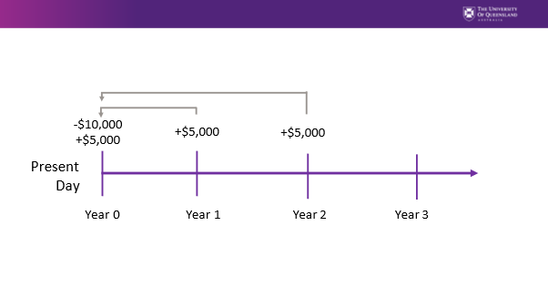
If we assume there is a project with an initial investment cost of $10,000 in year 0 and a net benefit for each year of $5,000 over a three-year period, the timeline for the project using end of year discounting will follow the following format described in Figure 3.1.
Figure 3.1: Timeline of an Example Project with Investment Cost of $10,000 and a $5,000 Benefit per Year for 3 Years.
Subsequently, the net benefit that occurs at Year 1 refers to the net benefit that occurs at the end of the first period we are accounting for in the project. Similarly, Year 2 represents the end of the second year and Year 3 represents the end of the third year the project runs. Remembering that the NPV formula is:
(1) 
Assuming a 5% discount rate, we can calculate the NPV for this project:

Beginning of Year Discounting
By convention, year 0 refers to the net benefit occurring right now. Therefore, if the benefits and costs are incurred at the beginning of the year the net benefit streams move forward in the timeline. If we consider the same $10,000 initial investment with the $5,000 of benefits occurring at the beginning of each year the timeline will look like:
Note that the net benefit stream received at the end of year 1 is the same as receiving a benefit at the beginning of year 2. Hence the formula from equation (1) can be adjusted to reflect this:
(2) 
Therefore, the NPV using beginning of year net benefit streams using a 5% discount rate can be found as follows:

From the formula, we can already observe that the NPV using beginning of year discounting is expected to be higher than using end of year discounting as we are using smaller discount factors. More specifically, we apply a discount factor of 1 to the initial investment cost and the first net benefit stream which is received at the beginning of year 1 (equivalent to year 0). The discount factor for year 2 would be  and the discount factor for year 3 would be
  . As the discount factors are higher for beginning of year discounting compared to end of year discounting, the NPV using beginning of year discounting will consequently be higher.
Mid-Year Discounting
Mid-year discounting is more common than beginning of year discounting as investment bankers often use this method to get a midpoint estimate for an investment choice. In CBA, this method is used when the benefit or costs are expected to occur over the course of the year.
(3) 
As suggested by equation 3, we are subtracting half a year from each time period discount using the midpoint of each year. If we consider the same $10,000 initial investment with the $5,000 of benefits occurring at the mid-point of year the timeline will look like:
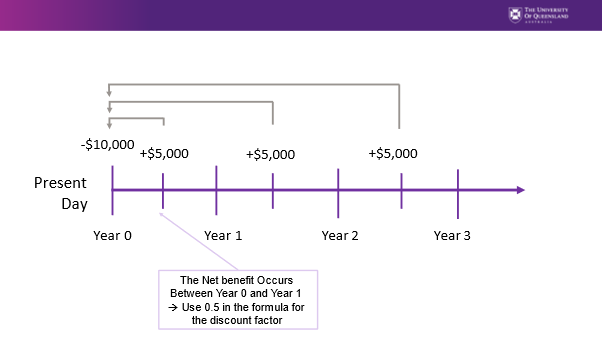
and the NPV using the midpoint formula can be calculated as follows:

Why Assume End of Year Discounting?
Discounting using the assumption of end of year impacts for both costs and benefits in the policy, project, or program being evaluated always provides a more conservative NPV. The idea is to “err on the side of caution” by using the end of year discounting method. Consequently, if the  for the end of year discounting method, it is implied that the NPVs would be larger for the mid-year and beginning of year discounting methods. This is illustrated in Example 3.1.
Example 3.1
Comparison of Results Using Excel


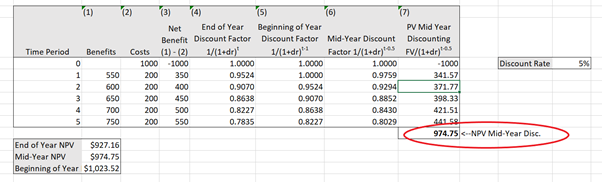
To calculate the NPV of each project in Excel you can use the “=NPV()” function for both End of Year and Beginning of year discounting. Remember that when using the “=NPV()” function for beginning of year discounting the values should start at year 2 for the appropriate discount factor to be applied. This will result in Excel treating the value from year 2 as a year 1 benefit stream to be discounted. Alternatively, you can calculate columns (4) and (5) to find the appropriate discount factor and multiply the net benefit in column (3) with the discount factor and sum the result.
Calculating mid-year discounting is more complicated as Excel is not set up for mid-year discounting calculations. Therefore, to calculate the result of mid-year discounting you can do it one of two ways:
(1) Calculate the appropriate discount factor for each of the time periods i.e., use  as shown in column (6). Then use the discount factor to calculate the present value of each net benefit, then sum these net benefits to get the correct result. i.e.

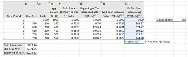
(2) Apply the formula in 3 directly to each net benefit stream as shown in column (6) and illustrated in Figure 3.4 to find the present value of each net benefit stream. After this, you only need to use the “=sum()” function to sum the column to calculate the NPV as shown in Figure 3.5.
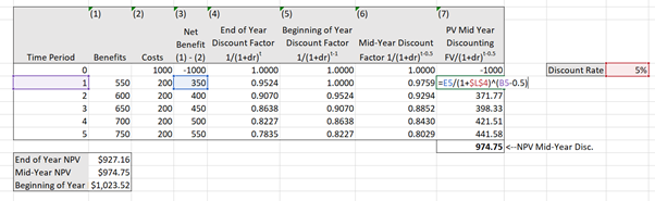
Click here to download the spreadsheet: Example_3_1.xls
Approximating Mid-Year Discounting
An alternative method that is sometimes adopted is to calculate the NPV under the beginning of year and end of year discounting methods and take the average of the two results. This gives a close approximation of mid-year discounting.
Example 3.2
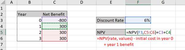
Approximate the mid-year discounted NPV using the average of the end and beginning of year results using the information in Table 3.2.
| Year | Net Benefit |
|---|---|
| 0 | -800 |
| 1 | 300 |
| 2 | 300 |
| 3 | 300 |
Assuming a 6% discount rate we can calculate the NPV using the beginning of year method as illustrated in Figure 3.7 below:
The end of year NPV can also be calculated as illustrated in Figure 3.8 below::
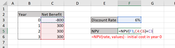
Taking the average of these results ($1.90 and $50.02 respectively) will give a value of $25.96 which is a close approximation of the mid-year discounted NPV.
To replicate this result and to practice beginning and end of year discounting you can download the spreadsheet here: Example3_2
See if you can replicate the result by calculating this by hand as well.
Comparing Projects with Different Time Frames
When comparing projects, it has been assumed that the period for the life of the project was equal. However, we know that this is not necessarily the case for real world decision-making as the NPVs of projects with different time frames are not directly comparable. For example, as CBA analysts we may be asked to compare the life of a road infrastructure project against a new solar farm. To make valid comparisons we look at two methods: (1) the equivalent annual net benefit (EANB); and (2) project roll-over. The choice of which method is most appropriate for comparison depends on whether it is possible to repeat a project investment.
Equivalent Annual Net Benefit (EANB)
The equivalent annual net benefit identifies a yearly annuity received for the life of a project. An annuity is a fixed sum of money paid or received per year. Common annuities include mortgage repayments or salary payments. Identifying the equivalent annual net benefit involves taking the NPV of the project and dividing it by the annuity factor to find a per year net benefit stream.
(4) 
Therefore, when you sum the total present value of the annuity series across the life of the project it must be equal to the total NPV of the project. Specifically,

where t is the number of years or life of the project.
By calculating the EANB, we determine the amount of net benefit received per year for the life of a project i.e., the yearly annuity benefit. Therefore, the sum of these annuity benefits will be equal to the NPV of the project under consideration.
(5) 
When comparing projects with unequal lives using EANB, we should select the project with the highest EANB – assuming we are not attempting to minimise net costs but seeking to maximise total net benefits.[1]
Annuity Factor
To effectively calculate the EANB in equation (4), we need to first calculate the annuity factor. The annuity factor is the sum of the discount factors over the life of the project where the stream of net benefits follows a fixed annuity format. As outlined in Chapter 2, the discount factor is:
(6) 
To demonstrate this relationship between the discount factor and the annuity factor, consider the following example in Table 3.3, with end of year discounting and a social discount rate of 6%:
| Year | Net Benefit | Discount Factor |
|---|---|---|
| 0 | -800 | |
| 1 | 400 | 0.9434 |
| 2 | 400 | 0.8900 |
| 3 | 400 | 0.8396 |
| AF = 2.6730 |
The discount factors across years 1 – 3 are:

Therefore, the annuity factor would be 2.6730. As can be seen from the example above, there is a geometric sequence with the common ratio of  . Therefore, we can summarise the annuity factor in the following equation:
(7) 
where  is the discount rate and
  is the number of years/life of the project.
Hence, the annuity factor represents the present value of an annuity of $1 per year for years when the discount rate is .
Key concept – Annuity Factor
The annuity factor represents the present value of an annuity of $1 per year for years when the discount rate is .
Substituting in the same values as before we can confirm the result for the annuity as follows:

This is reflected in the sum of the discount factors in Table 3.3.
Calculating the NPV of this project gives a value of $269.21. Therefore, applying equation (4), we calculate the EANB as $100.71. This EANB implies that the project has an equivalent annual benefit annuity of $100.71 per year across the three-year life of the project. Note that if we receive $100.71 per year across three years and then discount this benefit back at the same discount rate we will receive a total approximately $269.21 as highlighted in Table 3.4 below:
| Year | 0 | 1 | 2 | 3 |
|---|---|---|---|---|
| EANB Per Year (annuity stream) | 100.71 | 100.71 | 100.71 | |
| Discounted EANB | 95.01 | 89.63 | 84.56 | |
| NPV (sum discounted EANB) | 269.20 |
To replicate this example in Excel, you can download the spreadsheet here: Table3_4
Annuity Factor and EANB in Perpetuity
Key Concept – Perpetuity
A perpetuity is an annuity that has no end, or a stream of cash payments that continues forever.
When comparing projects with different time frames, we may come across the situation where a project does not have an end for the net benefit stream. This is known as a perpetuity. One thing we note about the annuity factor in equation (7), as the number of years increases (i.e.  ), the annuity factor in perpetuity becomes
  . Consequently, if we have two mutually exclusive projects A and B:
- Project A is a solar farm. It has NPV of $20 and a life of 25 years
- Project B is a hydroelectric plant has a NPV $30 million and continues in perpetuity.
We can calculate the EANB for both projects to compare which project should be selected. Assuming the appropriate discount rate is 4%, we calculate the annuity factor for Project A we apply equation (4) resulting in an  and a
and a  million per year across 25 years.
For project B we need to apply the annuity factor for a perpetuity . Therefore the  . Consequently, we then calculate the
  as
as  million per year in perpetuity.
From these results we can see that  therefore Project A should be selected.
We will see the implications of perpetuities for NPVs below.
Advantages and Disadvantages of EANB
Calculating the EANB is a good option for comparing projects with unequal lives as it annualizes the NPV allowing for a per year net social benefit comparison between projects on a per year common metric. Therefore, EANB can be used to rank projects and will subsequently provide a consistent decision when comparing projects with unequal lives.
The biggest limitation of the EANB method for project comparison is the selection of the discount rate. As shown in equation (6), there is an inverse relationship between the discount rate and the discount factor.
Example 3.3
Equivalent Annual Net Benefit Example
If we are considering two possible projects that are mutually exclusive:
- Project A: Benefit = $40,000 per year, Initial Cost = $ 15,000 in year 0, life = 3 years
- Project B: Benefit = $30,000 per year, Initial Cost = $ 10,000 in year 0, life = 4 years
If the appropriate discount rate is 5%. We can calculate the EANB for each project in three steps.
Step 1: Calculate the NPV of each project
In this case the values are already expressed in present values therefore we can take the difference between the PV(B) and PV(C).


Step 2: Find the annuity factor

And

Step 3: Calculate the EANB


As we are measuring net social benefit when comparing these projects, we select the project with the highest EANB. Hence, project A should be accepted as 
To complete this example in Excel, you can download the following spreadsheet: Example3_3
Example 3.4
One of the challenges of using Equivalent Annual Net Cost (EANC) instead of EANB is to remember that you are evaluating the cost effectiveness of a project. Therefore the net benefit stream will be negative. Therefore, you should select the project that minimises cost annuity. In this instance the project will still have the highest value, as the annuity calculated will be closer to zero. To see this, consider the following information on three mutually exclusive projects below:
| Project | NPV Cost | Life (years) |
|---|---|---|
| (1) | (2) | (3) |
| X | -3,500 | 2 |
| Y | -4,500 | 3 |
| Z | -6,000 | 4 |
Project X has a two-year life, Project Y has a three-year life and Project Z has a four-year life. The present value of each project across the life is already calculated for the first step in column (2).
The second step is to calculate the annuity factor for each project. Assuming the appropriate discount rate is 10% the annuity factor for a two-year project is 1.7355, 2.4869 for a three-year project and 3.1699 for a four-year project. Therefore, the EANC for each project can be calculated as below:


These results indicate that Project Y is the least costly option and therefore should be selected.
To replicate these results in excel you can download the spreadsheet here: Example3_4
Project Roll-over
The project roll-over method involves making the length of both projects the same by assuming the ability to “roll-over” or reinvest in the same projects repeatedly until an equal project life is achieved. This is often called the “common life” approach in capital budgeting.
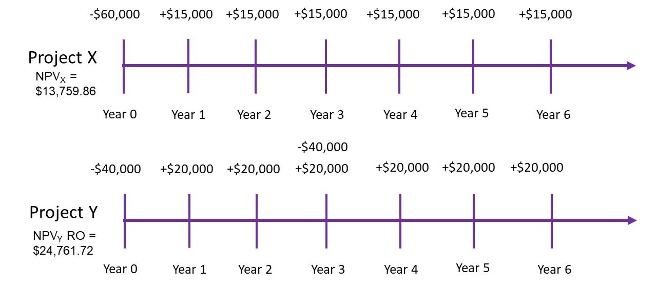
If we consider two projects:
- Project X – has a life of six years, an initial cost of $60,000 and a yearly net benefit stream of $15,000
- Project Y – has a life of three years, an initial cost of $40,000 and a yearly net benefit stream of $20,000
Assuming all benefits and costs accrue at the end of the year and the appropriate social discount rate is 6%, the project timelines and NPV for Project X can be illustrated as shown in Figure 3.9:
Figure 3.9: Timeline of Net Benefits for Project X.
Consequently, the NPV for Project X is found as follow:

The timeline for Project Y is different as the project only spans 3 years as illustrated in Figure 3.10:
Figure 3.10: Timeline of Net Benefits for Project Y.
Therefore, the NPV of Project Y is:

When the projects are considered mutually exclusive, the NPV decision rule implies we should accept Project X over Project Y. However, this decision is not correct as we know the projects, we are comparing have unequal lives. Therefore, if we assume Project Y can be rolled over and reinvested we can equate the timeline of Project Y to an equivalent time frame as Project X shown in Figure 3.11:
Figure 3.11: Timeline of Net Benefits for Project Y when the Project is Rolled Over.
Therefore the NPV of Project Y should be calculated as:

Following this, we can compare the two Project NPV’s with roll over in outlined in Figure 3.12. As can be seen from the project roll-over of Y the  is now higher than the
  when Project Y is rolled across the same number of years.
Alternatively, you can rewrite the formula for the NPV project roll-over as
(8) 
Where:
 the initial NPV of the project for the normal life span
 is the discount rate
 is the total number of periods required for roll-over
 is the initial project duration
Following the same example as above for Project Y:

This is also illustrated in Figure 3.13 below:
Figure 3.13: Applying the Roll-Over Method
Consequently, from the project roll-over approach – we should accept Project Y over Project X if the projects are mutually exclusive and reinvestment into Project Y is possible.
You can download the spreadsheet to complete this example Chapter3 Roll Over Example
In conclusion we can see from both the EANB method, and the Project Roll-over method illustrated in the sections above, we cannot just use the NPV decision rule when comparing projects with unequal lives. Instead, we should ensure we are comparing “apples with apples” by using either the EANB or roll-over comparisons depending on the assumptions around re-investment opportunities.
Other Complications in CBA
Real vs Nominal Values
One issue we often need to consider when conducting a cost-benefit analysis is whether to use real or nominal values to value the expected impacts. It is usually more convenient and less confusing to use real values (constant year 0 prices). Using nominal values requires the analysts to determine the prices of impacts in each year across the life of the project. In addition to this, when using nominal values, you should use a nominal social discount rate. This can add an additional layer of complexity to the analysis. When using real values, you can use the real social discount rate observed in year 0 for the life of the project. Following this approach, we adopt the use of “constant year 0 values” or “real values” as these are most appropriate for ex-ante CBA.
Key Concept – Real Values
For the purpose of this course, we assume real values at constant year 0 prices and the social discount rate at year 0 across the life of a project.
Dealing with Inflation and Growth
We know that benefits and costs of a policy, program, or project being evaluated often occur in the future. By using real terms for evaluation of the project under consideration, we neutralise the impact of inflation in the analysis as all impacts are measured in a constant year 0 price. For practical purposes, it is safe to assume that the prices will remain relatively constant to all other aspects of the economy, so unless we expect the sector under evaluation to experience rapid disproportionate changes relative to the rest of the economy, it is reasonable to use real terms to ignore inflation.
Financial appraisal usually deals with the issue of inflation. Usually, we are approaching the evaluation of public projects from a social perspective, which implies inflation can be ignored to an extent. However, it is important to ensure that we can account for inflation where necessary when a private firm is involved in the project. Consequently, it is important to note that from a financial appraisal perspective the discount rate is often substituted with the real interest rate for an investment and the analysis will capture the impacts of inflation on a project. Therefore, it is important to understand the relationship between nominal and real interest rates. In a project appraisal, a private firm may adjust the cashflows of a project using the following real interest rate formula:
(9) 
where
 the real interest rate
 the nominal interest rate
 inflation rate
In the context where evaluation of a project occurs over many periods with large values, it is not considered appropriate to use the approximation formula as it may impact the NPV calculations.
It is usual to undertake ex-ante CBAs in real terms and financial appraisals in nominal terms. Also note that when conducting an ex-post CBA we use the nominal prices that were observed in the past. This allows the analyst to determine the precision of the results and provides an opportunity to refine future CBAs.
Key Concept – Discount Rate versus Interest Rate
The discount rate in social cost-benefit analysis is different to the interest rate used in financial appraisals and therefore we often ignore the implications of inflation on the project evaluation.
Example 3.5
If the nominal interest rate is 5% and the inflation rate is 2%, we can calculate the real interest rate as:

Example 3.6
Suppose we have an investment that provides a real net benefit of $230 per year over 5 years, at a cost of $1,000 at the beginning of the project.
If the inflation rate is expected to be 5% each year over the life of the project, we can calculate the nominal net benefits in each year.
| Year 0 | Year 1 | Year 2 | Year 3 | Year 4 | Year 5 | |
|---|---|---|---|---|---|---|
| Net Benefit (Year 0) | -1,000 | 230 | 230 | 230 | 230 | 230 |
| Net Benefit (Nominal – Current Year) | -1,000 | 241.5 | 253.58 | 266.25 | 279.57 | 293.54 |
Calculating the internal rate of return, we get a nominal IRR of = 10.1% and NPV of $118 when we assume a 6% discount rate. When using current year prices (i.e. year 0 prices), we get the real IRR of 4.6% and an NPV of -$31.
In some cases, this would lead an investor to believe that the rate of return is better for the project under nominal terms. However, this is not true. It is the same project! The measurement is just different as we have expressed the net benefit in nominal terms compared to real terms. Consequently, we need to be cautious when using nominal values for our analysis.
If we were using an IRR rule, we need to ensure that we compare the cost of capital in real terms when using real values or nominal terms when using nominal values. Therefore, we would need to use the formula in (9) to adjust between real and nominal values.
To practice calculating the NPV and IRR you can download the spreadsheet for this example here: Example3_6
Horizon/Terminal Values
We usually assume that the benefits and costs of a project are accrued over a set time frame. However, when it comes to capturing social costs and benefits, we are likely to experience impacts into the future, beyond the life of the project. When we consider policies where benefits and costs that may continue past the scope of evaluation, we need to ensure we capture these impacts in our social cost-benefit analysis. For example, if the government implemented a program that involved early childhood reading activities in pre-school care programs, the benefits from the intervention would likely impact the children involved in the program across their whole life and even potentially produce intergenerational impacts. However, the scope of evaluation for a program such as this would not be conducted across the lifetime of the individuals involved. Instead, the program or intervention would be evaluated within the timeframe set by the relevant government department.
This idea of impacts observed beyond the time frame used for the evaluation of a project is important. When conducting a social cost-benefit analysis, there is an expectation that the analysis captures all social costs and social benefits to ensure the accuracy of the results. Therefore, we as analysts face a challenge in measuring these potential benefits and costs. The solution to this is to utilise horizon values. Depending on the approach to social cost-benefit analysis for the project under evaluation, there are different methods for capturing the horizon value.
From a social cost-benefit perspective, the best approach is to calculate the benefits and costs accruing for the project in the form of a final expected benefit which can be discounted to the present. We can therefore calculate the appropriate NPV the following two ways:
- Calculate the horizon value for the relevant duration and discount the horizon value to the present using the appropriate duration. i.e.
 . Such that
  where is the appropriate duration for which the benefits and costs will accrue into the future.
 - Calculate the horizon value and treat it as a perpetuity i.e.,
 . This method is useful when a duration cannot be effectively determined.
From a financial appraisal perspective, the salvage value (sometimes referred to as residual value or scrap value) can be used as a proxy for the horizon value. This salvage value usually occurs in the last year of a project and requires discounting. Consequently the NPV of a project is therefore calculated as the 
 . This is a common approach in transportation and infrastructure evaluations. However, this approach assumes that market prices reflect the true social value of the underlying project being evaluated. In real world applications, salvage values can be positive or negative depending on whether the project investor would receive a positive cash flow from on-selling the remnants of the project or whether there is a cost associated with disposing the remnants of the project. For example, a factory may sell their machinery at the conclusion of the project for a positive salvage value whereas mining projects often have a salvage cost for land rehabilitation.
Key Concept – Salvage Value
Salvage Value is usually treated as a “negative cost” and not necessarily a positive benefit – implying a positive inflow for salvage that is accounted for in the cost section of an evaluation. Consequently, it will impact the BCR of a project if the salvage value is sufficiently large.
In some instances, the horizon value is set to zero. This approach assumes that there are no benefits and costs accruing to a project after the time frame used in the evaluation. This is the easiest method for dealing with the horizon value issue, however important benefits and costs may not be included in the social cost-benefit analysis. Consequently, the NPV may be underestimated or overestimated. For example, if we were considering the same government implemented for early childhood reading activities the NPV would likely be underestimated as the lifetime increases in earnings of participants would not be captured outside of the stated time frame. Therefore, although this is the easy method it can result in an inefficient allocation of the scarce resources.
Consequently, the decisions relating to how we approach horizon values need to be carefully considered when conducting a social cost-benefit analysis.
Example 3.7
Consider the following project
The initial cost is $10,000
Annual Benefit of $6,000
Immediate life of the project for evaluation is 3 years. Smaller spill over benefits are expected to accrue into the future over a 20-year period to the value of $1,500 at the end of year 20. If the discount rate is 5%,

Example 3.8
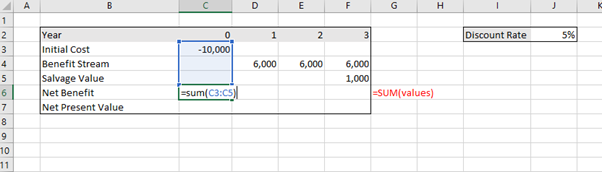
Consider the same information as Example 3.7 above replicated in Table 3.6 below. Suppose instead of using a horizon value, we calculate a salvage value equal to 10% of the initial cost of investment. The immediate life of the project for evaluation is 3 years. Salvage occurs at the end of the project. If the discount rate is 5% we can determine the following:
| Year | 0 | 1 | 2 | 3 |
| Initial Cost | -10,000 | |||
| Benefit Stream | 6,000 | 6,000 | 6,000 | |
| Salvage Value | 1,000 |


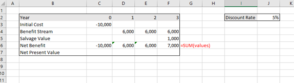
To calculate this in Excel you can use the “=sum()” function to calculate the net benefit stream (shown in Figure 3.14). After pressing enter, you will have the sum of column C.
You can copy the formula across using the black plus symbol that appears when you hover at the bottom right corner of the cell “+” and Excel will calculate the same formula for each column as shown in Figure 3.15.
Once this is complete, you can apply the “=NPV()” function as illustrated in Figure 3.16:
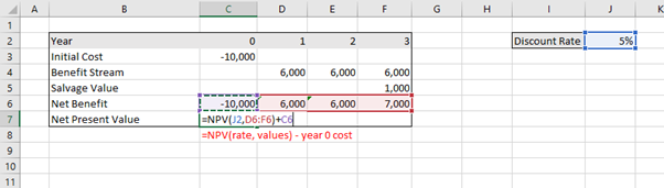
To replicate this result, you can download the spreadsheet here: Example3_8
Present Values in Perpetuity
The final aspect we need to consider was briefly mentioned when discussing horizon values as above. Some horizon values can be considered in perpetuity. If a benefit or cost is expected to accrue in perpetuity, we need to be able to calculate the present value of the perpetuity. To do so we apply the following formula:
(10) 
Key Concept – Perpetuity
A perpetuity is a constant flow that occurs forever.
It is important to note that the present value of a perpetuity is not significantly different from the present value of an annuity over a long period, however it applying a perpetuity formula allows for a more conservative NPV estimation when applied to horizon values or similar issues that need to be accounted for in CBA.
Example 3.9
Suppose there is a perpetuity benefit of $250 per year. Assuming the appropriate discount rate is 10%, the present value of the benefit would be

Suppose instead of assuming the benefit is in perpetuity and instead we apply a 35- year duration we calculate the PV of the benefit as

NPV in Perpetuity with Growth
If we also require the growth rate to be accounted for in our perpetuity calculation, we adjust the formula as follows:
(11) 
However, CBA analysts often do not capture growth or inflation in the analysis as the preference is to use, constant real year 0 values to reduce complexity.
Revision
The Excel spreadsheet for the above question can be downloaded here: Chapter3Revision_Q2
The Excel spreadsheet for the above question can be downloaded here: Chapter3Revision_Q5
Summary of Learning Objectives
- The assumption that all costs and benefits are realised may not be appropriate for all projects. Therefore, it is important to be able to apply beginning and mid-year discounting.
- When comparing projects with unequal timeframes, we can apply either the rollover method or the equivalent annual net benefit method. The assumptions of these methods are different.
- We need to include scrap/ salvage values or horizon values to capture benefits or costs that persist after the evaluation period of the project. This is especially important if the horizon value or scrap value will significantly impact the net present value.
- Some projects run in perpetuity and therefore it is appropriate to evaluate those projects using the perpetuity formula.
- Alternatively if the project only runs at a cost, we can calculate the equivalent annual net cost and select the project which minimises the cost. ↵
