
Chapter 2: Decisions, Decisions, Decisions.
Learning Objectives
After completing this chapter, students should be able to:
-
Explain why it is necessary to discount in cost-benefit analysis.
-
Implement discounting over single and multiple periods.
-
Calculate the NPV, IRR, and BCR.
-
Utilise decision rules to identify worthwhile projects using NPV, IRR, and BCR methods.
Introduction
In this chapter we want to be able to identify the net social benefit for any policy, project, or program under consideration in a cost-benefit analysis. Remembering the net social benefit is the welfare derived from the policy, program, or project under consideration, there are three key methods (or criterion) for estimating the Net Social Benefit of a project in CBA:
(1) Net Present Value,
(2) the Internal Rate of Return, and
(3) Benefit-Cost Ratio
We will look at each method consecutively. But first we need to understand key concepts that capture social time preferences within the confines of cost-benefit analysis. Then, we will look at the three methods for finding the net social benefit. We will conclude this chapter with a framework that allows us to compare between project choices. This is particularly important when projects are potentially mutually exclusive.
Time Preferences and Net Social Benefit
As we defined in the first chapter the net social benefit is the difference between the total social benefits and the total social costs:
(1) 
Let us consider an example:
Assume a company is interested in purchasing a new software. The initial capital investment of $10,000 is required to purchase the software. The expected benefit to the company is an increase in productivity of $25,000. Therefore, we can calculate the net benefit to the company as NB = $25,000 – $10,000 = $15,000. Since the net benefit to the company is positive, the company should purchase the software. This assumes that the purchase of the software experiences no market failures.[1]
However, we know that benefits and costs of a project may not occur in a single period and therefore the analysis of net social benefit is not static in most cases. Projects, programs, or policies can have short-term impacts or long-term impacts. It is critical to account for the period of time in which the benefits accrue. If we consider the example from before whether the company purchases software, it would be safe to assume that the company would continue to receive benefits from the software into the future and not just once off.
Let us assume the company does not receive a benefit of $25,000 up front and instead received a benefit of $25,000 in 5 years. This introduces an element of time into our decision-making process. With this addition of time there is an element of uncertainty. Therefore, the value of a sum of money should be valued differently depending on when the cash flow occurred.
Time Value of Money
The time value of money demonstrates that all things being equal, a dollar today is worth more than a dollar in one year. Even if there is no inflation, a dollar today can be used productively to ensure that it yields a greater value in the future. Therefore, there is an opportunity cost that is associated with the time you wait to receive money.
Consequently, we cannot compare dollar values that accrue or occur at different points in time. Our solution to this problem is compare costs and benefits over time by discounting.
Discounting
Following from the implications of the time value of money, a key element of cost-benefit analysis is the evaluation of costs and benefits that occur over time. This evaluation is known as discounting.
Discounting is the methods we use to consider the benefit and costs that accrue progressively. Discounting refers to the process of estimating the present value of a future cash flow or monetary values. Traditionally, in CBA we discount all benefits and costs into the present value as it provides a common metric for comparison. This means we express the monetary values received throughout the life of a project at the same point in time.
Discounting is a key element in valuing future benefits and cost within a cost-benefit analysis framework. By discounting the expected value of benefits and costs, we can determine if giving up some consumption benefits today yields greater benefits in the future. Therefore, the need for discounting arises from opportunity costs in CBA.
Key Concept – Benefit and Cost Streams or Cash Flow?
For the purpose of this course, it is a good idea to view the accrued benefits and costs as “cash flows”. When we refer to cash flows in this book, we are referring to the monetised values of tangible and intangible benefits and costs. Therefore, although we use the term cash flow, the dollar values may not reflect the market prices.
We will use the terms cash flow and benefit/cost streams interchangeably.
Discount Rate
To be able to calculate the present value of a benefit or cost we need to determine the appropriate discount rate. Often in financial appraisals the choice of discount rate is the prevailing interest rate for investors, as it captures the opportunity cost of investing. However, in a cost-benefit analysis, the discount rate represents more than an interest rate. The discount rate should capture the preferences for consumption, social time preferences, and relevant opportunity costs. Therefore, the discount rate used in cost-benefit analysis should be higher than the interest rate used in financial appraisals. Consequently, we refer to the discount rate used in social cost-benefit analysis as the “social discount rate”.
It is also important to note that there is no one single discount rate that is used for all projects in social cost-benefit analysis. This is due to different policies having different opportunity costs.
Key Concept – No single social discount rate
The discount rate is often different depending on the type of projects being evaluated. For example, the choice of social discount rate for evaluation of climate change mitigation policies would be significantly different to those social discount rates used in transportation infrastructure.
It is of utmost importance to ensure you select the appropriate discount rate for estimating present or future values. The choice of discount rate can make a significant difference to whether the project is positive or negative. It also impacts the relative desirability of projects when costs and benefits accrue at different times or over different project lives.
So, by discounting using the social discount rate we can compare the costs and benefits at different points in time within a common metric, either in the present or future.
Present Value
As we now understand the components required for discounting, we can implement the present value formula to calculate the present discounted value of benefits and costs. The present value is the value of a stream of benefits or costs at the date of evaluation in the project i.e., the current year.
For a single period the present value formula is:
(2) 
where  is the present value,
  is the future value of the benefit or cost stream and
  is the social discount rate.
Example 2.1:
Assume we have a future benefit stream of $10,027.50 in a year’s time (year 1) and a social discount rate of 5%. We can calculate the present value of the benefit in present terms (in year 0) as follows:

When comparing between mutually exclusive projects we would select the project with the largest present value.
Click through the slideshow below to see the steps involved in calculating the present value from Example 2.1.
Future Value
As we are interested in expressing the cash flows in a common metric, an alternative method is to calculate the future value. This process is also known as compounding. A future value is the value of a current benefit or cost stream at some date in the future. To calculate the future value, we can rearrange the formula we had for the present value:
(3) 
Example 2.2
Assume we have a current cost stream of $9,000 (at year 0). We would like to calculate the future value of that $9,000 cost in a year’s time (end of year 1) using a social discount rate of 5%. Substituting in the values will give:

Therefore, the future value tells us how much the benefit or cost stream observed today would be worth in the future.
Click through the slideshow below to see the steps involved in calculating the future value from Example 2.2.
Multiple Period Discounting & Compounding
In the above examples we assume a single period for discounting and compounding. However, we know that benefits and costs accrue over long periods of times. We can extend our formulas for calculating the present value and the future value fairly easily.
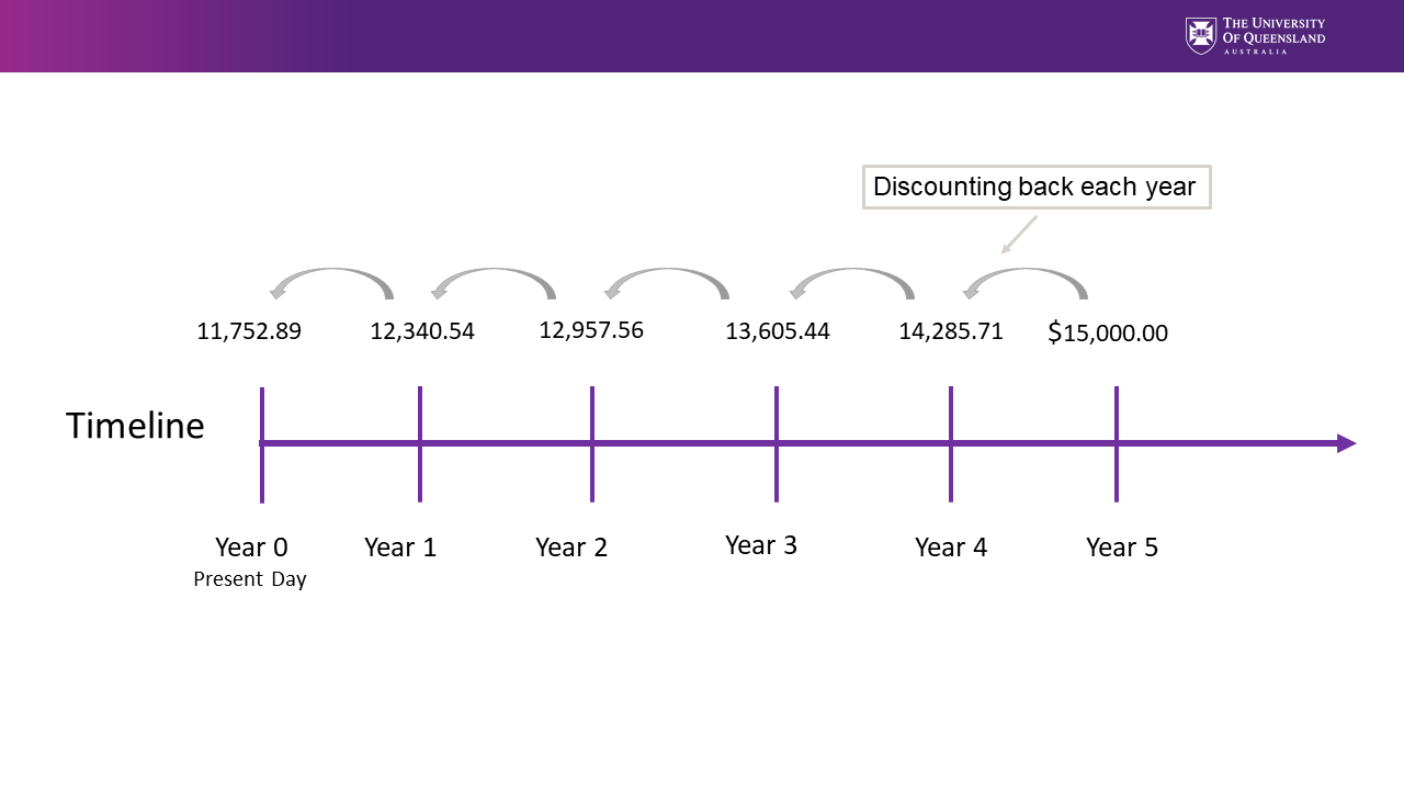
Assume there is a benefit stream of $15,000 that is realised after 5 years, and the social discount rate is 5%.
We can use our present value formula to move our benefit back in time from Year 5 to Year 4.

Therefore we have moved the value of the benefit stream to an equivalent value for Year 4. We can do the same thing to move the Year 4 value to Year 3.

Continuing this process to move towards the present value at Year 0, you would get the results in the Table 2.1 (and illustrated in Figure 2.1)


![PV_3 = PV_4/ (1+0.05) = [$15,000/(1+0.05)]/(1+0.05) = $15,000/(1+0.05)^2](https://uq.pressbooks.pub/app/uploads/quicklatex/quicklatex.com-d8d7100c6478a0761f235dd2f6a739dd_l3.png "Rendered by QuickLaTeX.com")


![PV_2 = PV_3/ (1+0.05) =[$15,000/(1+0.05)^2]/(1+0.05) = $15,000/(1+0.05)^3](https://uq.pressbooks.pub/app/uploads/quicklatex/quicklatex.com-da9fcc96e9d74785878671f77238d4b7_l3.png "Rendered by QuickLaTeX.com")


![PV_1 = PV_2/ (1+0.05) =[$15,000/(1+0.05)^3]/(1+0.05) = $15,000/(1+0.05)^4](https://uq.pressbooks.pub/app/uploads/quicklatex/quicklatex.com-7117307f5f04d895f75b2c6ee25f5da9_l3.png "Rendered by QuickLaTeX.com")


![PV_0 = PV_1/ (1+0.05) =[$15,000/(1+0.05)^4]/(1+0.05) = $15,000/(1+0.05)^5](https://uq.pressbooks.pub/app/uploads/quicklatex/quicklatex.com-c0fa6e722ea9ee552010a6268a8a230c_l3.png "Rendered by QuickLaTeX.com")

From Table 2.1 above we can see that calculating a multi-period present value is a iterative process. The derived formula for discounting can therefore be written as:
(4) 
where  is the number of years before the benefit or cost is realised and
  is known as the discount factor.
To confirm this result, we can apply the formula to our example above where  years:

In CBA we mostly deal with present values for our analysis. However, we may also need to compute the future value. To find the future value over multiple periods, we can rearrange the result from (4) to get the following formula:
(5) 
Future value often used to account for growth or inflation by replacing the discount rate () with the relevant growth or inflation rate. These future values are then usually discounted back into the present value.
Conventions for Benefit and Costs Streams
The initial or present period is always referred to as year 0. Year 1 is one year from the present year. Unless otherwise stated we assume that benefits or costs accrue on the last day of the year. However, we can also conduct mid-year and beginning of year discounting by adjusting the formula. A discussion of mid-year and beginning of year discounting can be found in Chapter 3.
Key Methods for Estimating Net Social Benefit
There are three key methods for estimating the Net Social Benefit of a policy, program, or project. Each method requires all social costs and benefits to be accounted for in the application of the formula. If benefits and costs are not correctly identified, predicted, and monetised, this can potentially lead to the incorrect conclusion relating to the project.
Net Present Value
Now we understand present value and future value, we can use this information to calculate the net present value. The Net Present Value (NPV) is useful for dealing with multiple time periods and numerous benefits and costs may be involved in a policy, program or project. In its simplest form the net present value is:
(6) 
A useful expression for computing the net present value over multiple time periods is:
(7) 
Or alternatively if  in each given year:
(8) 
where you take the difference between the benefits and the costs in each period.
Example 2.3
Suppose a project under consideration has an initial investment cost of $1,000. The project is expected to yield a benefit stream of $300 per year for 5 years and has an ongoing cost of $50 per year for the life of the project. This information is summarised in Table 2.2 below.
If we apply the first method of calculating the net present value based on equation (7) we start by calculating the present value of each benefit stream in column (4). Then we calculate the present value of the cost stream per column (5). Then you take the total sum of the present value of the benefits and subtract the total sum of the present value of the costs. The difference is the NPV of the project valued at $53.09.
Alternatively, per equation (8) the NPV can be found by taking the difference between the benefits and the costs to find the net benefit shown in column (6). After this step you calculate the present value of each net benefit in a given year, summing them up will give the net present value of $53.09. Note that both methods result in the same answer. However, the second method using the net benefits is more commonly used in spreadsheet applications.
Finding the NPV using Excel
To make our lives easier, we can use Excel to calculate the NPV of a project using the =NPV() function. The =NPV() function will calculate the net present value of future benefits and/or costs from year 1 onwards. Any costs or benefits accrued in the present year (year 0) should not be captured in the function.
The NPV function can be used in consecutive row or columns as illustrated in Example 2.4 below.
Example 2.4
Consider project Y which has an initial cost of $800 and a yearly benefit of $300, summarised in Table 2.3:
| Year | Net Benefit |
|---|---|
| 0 | -800 |
| 1 | 300 |
| 2 | 300 |
| 3 | 300 |
Assuming the appropriate discount rate is 6%, we can implement the NPV function using the =NPV() command as illustrated in Figures 2.2 and 2.3 below. i.e., =NPV(discount rate, series of benefits/costs that require discounting).
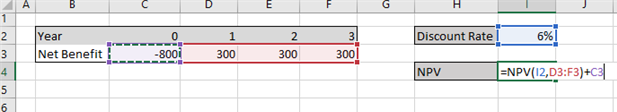
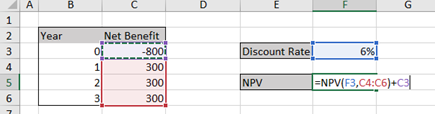
Note that the discount rate is highlighted first, followed by the cashflows from year 1 onwards. Cashflows from year 0 need to be either added or subtracted depending on whether it is a cost or a benefit. In this case we have a cost in Year 0 in the Excel spreadsheet inputted as -800 and therefore, to subtract it from the present value of the cashflows (highlighted in red) we will need to add it back (i.e., a positive number plus a negative number gives a negative number).
The result is an NPV = $1.91.
To replicate this example you can download the spreadsheet found here: Example2_4
Net Present Value Decision Rule
Based on our definitions for allocative efficiency outlined in Chapter 1, we should undertake any project where the  as there is a potential for pareto improvement. We refer to this as the NPV criterion. However, the decision rule for determining the highest net social benefit using the NPV decision rule is not that simple.
Key Concept: Decision Rules
A decision rule outlines the scenarios where we would accept or reject a project, program, or policy we are evaluating within our cost-benefit analysis framework. [2]
We have three possible scenarios for which we need to identify the NPV decision rule:
- Considering one project in comparison to the status quo.
When a single project is compared to the status quo, the decision rule is simple. If the the project should be undertaken as the net social benefit is greater than zero and the evaluation framework has identified a potential for pareto improvement as the present value of the discounted benefits exceeds the present value of the discounted costs. If the  reject the project in favour of the status quo. A NPV less than zero would indicate that the project is detrimental to society and has a negative impact overall.
- Considering multiple projects that are mutually exclusive.
If you are completing a cost-benefit analysis on a series of mutually exclusive projects, the project with the highest NPV should be selected. The project with the highest NPV is considered the most allocatively efficient outcome from the set of potential projects. However, if the for all alternative projects, reject the projects in favour of the status quo.
Key Concept – Logic of the NPV decision rule
The NPV identifies the monetised net benefit as an equivalent of today’s cash. Consequently, when comparing NPVs, we select the alternative with the highest NPV.
- Considering multiple projects that are not mutually exclusive.
When comparing projects that are not mutually exclusive, decision rules can become more complex. We can see this illustrated in Table 2.4 below. If there were no budgetary constraints, we would undertake all projects with a positive NPV. This would be projects A, B, D and E. Following our NPV criterion, we would not undertake project C as it is not a valuable use of our resources as it has a negative NPV.
However, in the real world we are often limited by a budget constraint sometimes referred to as capital rationing. In this instance it is best to take a capital budgeting approach to the cost-benefit analysis decision. In the instances where there is a budget, Stokey and Zeckhauser (1978) suggests that projects should be ranked by the ratio of net benefit to capital cost. This is the same as calculating the ratio of net present value to capital cost when net present value is our method of choice to approximate net benefits. Note that this method is different to calculating the benefit-cost ratio as it utilises the initial capital investment in the project rather than all associated costs. Once ranked, analysis should undertake projects in ranked order until budget exhausted. This is under the assumption that projects are indivisible in the context of social cost-benefit analysis.
However, the best approach from an economic perspective should utilise the NPV as it represents the best allocation of resources to society. The result is heavily influenced by the available budget. For example:
- Budget = $900 – undertake projects A and B which would expend the full budget and receive the highest total net present value.
- Budget = $1,000 – undertake projects A, B and E which would expend the full budget and receive the highest total net present value.
- Budget = $500 – project B should be selected over project A and E combined as it would provide the largest net present value.
Net Present Value and the Choice of Discount Rate
Selecting the correct discount rate is critical for the decision rule. The choice of discount rate will determine whether a project is accepted or rejected. As the discount rate increases, the net present value decreases.
Typically, when considering social cost-benefit analysis, a policy or program involves a large upfront cost followed by benefits accruing at a later date. When benefits accrue later in a project – the lower the discount rate the more attractive the project will be as the net present value will be much higher. If we select a higher discount rate than necessary, a desirable project may be rejected. Alternatively, if the selected discount rate is too low this may result in an undesirable policy or project may be accepted. See Example 2.5 below.
Example 2.5
Suppose we are considering two mutually exclusive projects A and B with the stream of net benefits summarised in Table 2.5. The projects have the same initial investment cost of $15,000. The difference between the projects is the size of the benefits over time. The benefits of project A decrease over time and the benefits of project B increase over time.
| Year | Project A | Project B |
|---|---|---|
| 0 | -15,000 | -15,000 |
| 1 | 6000 | 1500 |
| 2 | 5000 | 2500 |
| 3 | 4000 | 3500 |
| 4 | 3000 | 4500 |
| 5 | 2000 | 5500 |
| 6 | 1000 | 6500 |
From our NPV equation identified in (7), we know there is a negative relationship between the net present value and the discount rate. This is illustrated by a downward sloping curve in Figure 2.4.
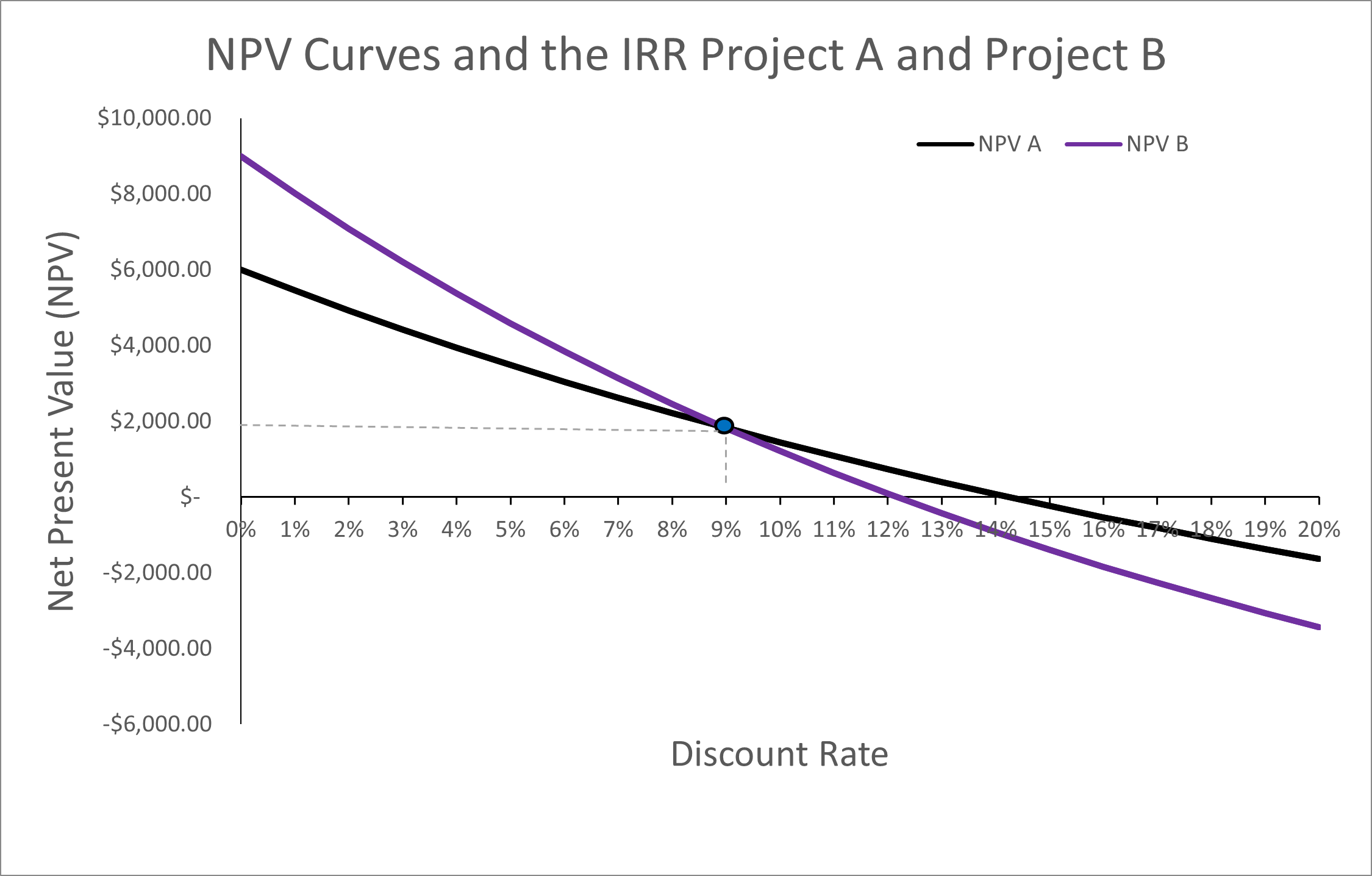
Figure 2.4: NPV Curves for Projects A and B
If we assume the appropriate discount rate is 5% for the project, we would choose project B over project A as NPV B ($4,581.53) > NPV A ($3,486.16). Alternatively, our decision rule would indicate the project A should be accepted over project B if appropriate discount rate was 12%. This change in preferences can be confirmed when we plot the NPV curves for project A and project B on the same graph in Figure 2.4.
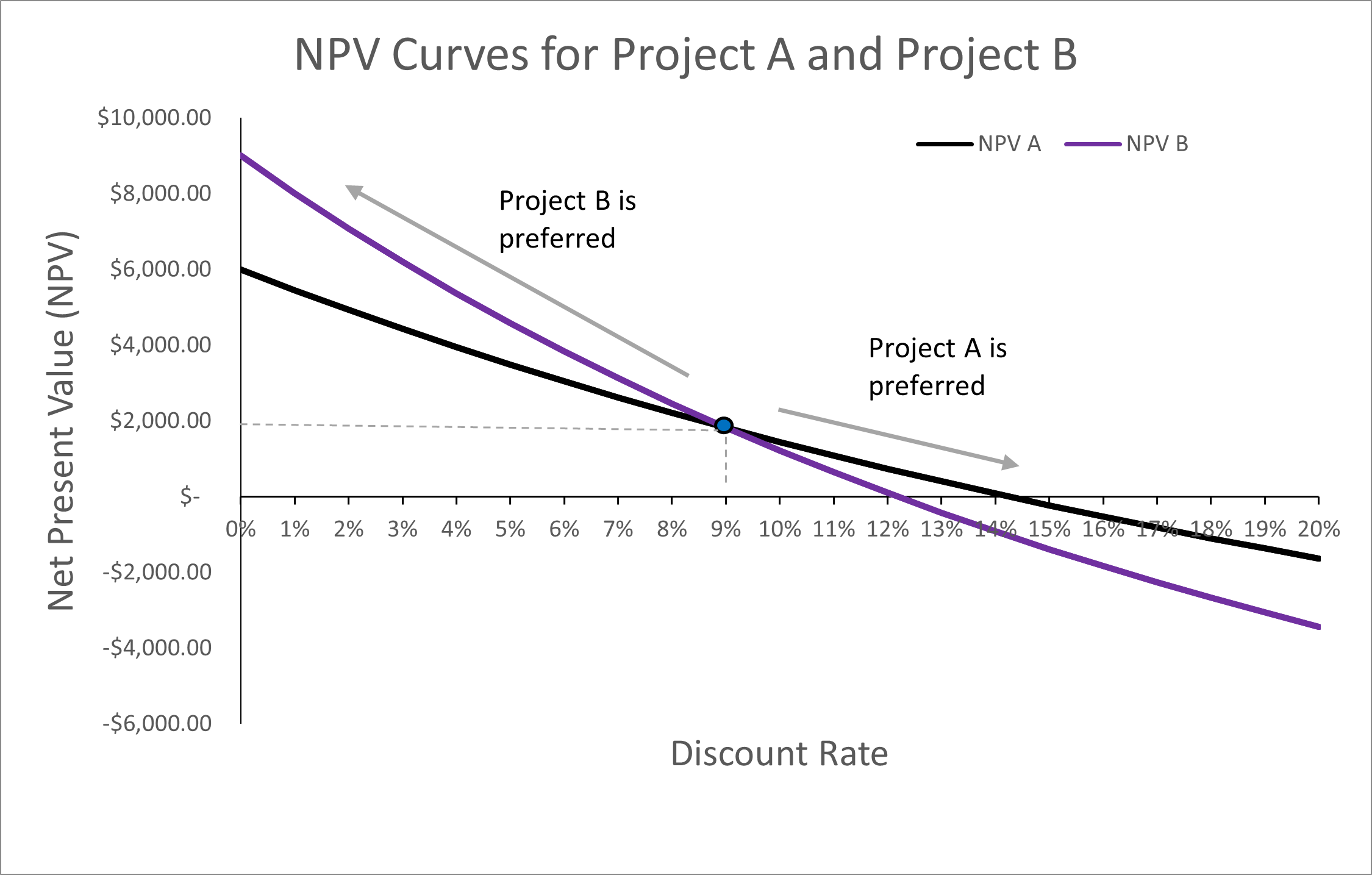
As highlighted in Figure 2.5, when we plot both project A and project B on the same graph we can see that project B is preferred to project A at all discount rates between zero and 9%. Once the discount rate is above 9%, we should choose project A over project B. This illustrates how the timing of benefits interacts with the discount rate. When the discount rate is sufficiently high, the preferred project will be the project with the larger cashflows upfront. More specifically, we see in Figure 2.5 the point where the preferences for which mutually exclusive project we would accept switches. This is known as the crossover rate or switching rate. At this point the NPV of project A and Project B are equal, and we are indifferent between the two projects. As illustrated in the figure, this occurs at 9%.
We know that Project B has a steeper NPV profile. This suggests that Project B is more sensitive to changes in the discount rate compared to Project A. Remembering that the benefits of Project A decrease over time and the benefits of Project B increase over time – we can see that discount rates above the switching point result in preferencing Project A. This is due to inverse relationship between the NPV and the discount rate. The higher the discount rate the lower the present value of future net benefits. Therefore, if the discount rate is high project A is preferred as the net benefits are accrued earlier in the project relative to the net benefits accrued to Project B which occur later in the project. Therefore, we can see that in this case a high discount rate indicates a preference for larger cash flows up front.
Advantages of the NPV Decision Rule over other Decision Rules
The advantage of the NPV decision rule is the clear monetisation of the costs and benefits in today’s monetary terms. It provides a practical measure of the magnitude of the net benefits as a monetary value. Further to this, the NPV decision rule provides a clear decision criterion for comparison.
Limitations of the NPV Decision Rule
The main limitation of the decision rule is it relies on the selection of the appropriate discount rate. It is possible that a change in the discount rate may lead to a change in the decision rule. Consequently, CBA analysts often look at the sensitivity of the NPV to a series of discount rates. This is known as a sensitivity analysis and will be covered in depth in Chapter 10.
The Internal Rate of Return
An alternative to the NPV approach is to calculate the internal rate of return (IRR) for policy, project, or program. The internal rate of return is discount rate in which the NPV is zero. This implies that the IRR is the discount rate where the sum of the discounted benefits is equal to the sum of the discounted costs. i.e.,
(9) 
This can also be expressed as:
(10) 
We can effectively find the IRR in two ways:
- 1) Graphically
- 2) Using the =IRR() function in Excel
Finding the IRR graphically:
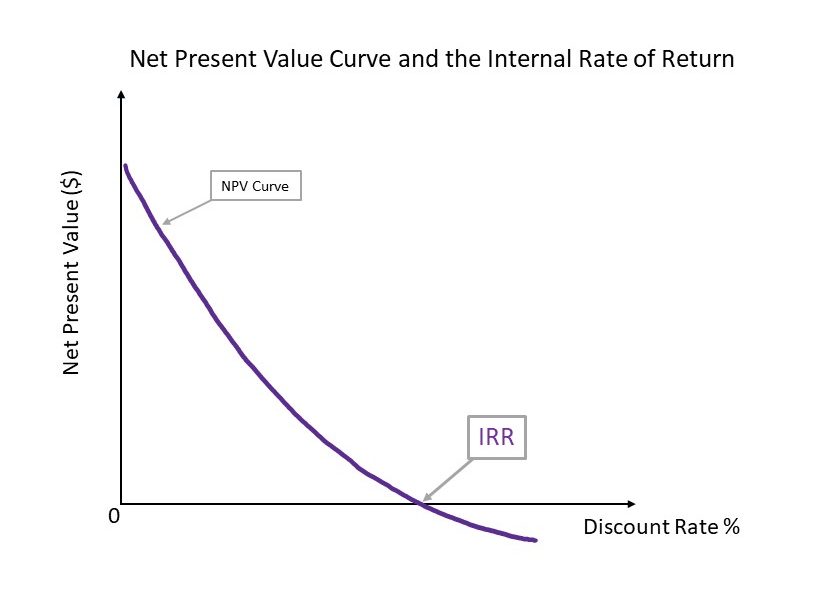
As mentioned before, the IRR is the point where the NPV is zero. This can easily be identified on the relevant NPV curve by looking at where the curve intersects the horizontal axis (i.e., where NPV = 0 on the vertical axis, shown in Figure 2.6). However, this method only provides an approximation of the IRR.
Finding the IRR using Excel:
Using the “=IRR()” function in Excel and highlighting the cashflow series from time zero onwards will provide the IRR.
Example 2.6
Following from Example 2.5 replicated below:
| Year | Project A | Project B |
|---|---|---|
| 0 | -15,000 | -15,000 |
| 1 | 6000 | 1500 |
| 2 | 5000 | 2500 |
| 3 | 4000 | 3500 |
| 4 | 3000 | 4500 |
| 5 | 2000 | 5500 |
| 6 | 1000 | 6500 |
Calculating the NPV’s across a range of discount rates and then plotting in a graph will allow us to identify the IRR for Project A and Project B respectively. This identifies the NPV profile of each project.
| Discount Rate | NPV A | NPV B |
|---|---|---|
| 0% | $ 6,000.00 | $ 9,000.00 |
| 1% | $ 5,452.35 | $ 8,013.72 |
| 2% | $ 4,928.46 | $ 7,082.28 |
| 3% | $ 4,426.95 | $ 6,201.98 |
| 4% | $ 3,946.58 | $ 5,369.45 |
| 5% | $ 3,486.16 | $ 4,581.53 |
| 6% | $ 3,044.59 | $ 3,835.34 |
| 7% | $ 2,620.86 | $ 3,128.19 |
| 8% | $ 2,214.00 | $ 2,457.59 |
| 9% | $ 1,823.13 | $ 1,821.26 |
| 10% | $ 1,447.39 | $ 1,217.06 |
| 11% | $ 1,086.02 | $ 643.01 |
| 12% | $ 738.27 | $ 97.28 |
| 13% | $ 403.46 | -$ 421.84 |
| 14% | $ 80.95 | -$ 915.94 |
| 15% | -$ 229.88 | -$ 1,386.50 |
| 16% | -$ 529.60 | -$ 1,834.88 |
| 17% | -$ 818.73 | -$ 2,262.38 |
| 18% | -$ 1,097.79 | -$ 2,670.19 |
| 19% | -$ 1,367.25 | -$ 3,059.42 |
| 20% | -$ 1,627.55 | -$ 3,431.12 |
Finding the IRR graphically:
Using the information above, the NPV curve of project A intersects the horizontal axis at approximately 14%. Therefore, the IRR for project A is approximately 14% as this is where the NPV is equal to zero (measured by the y axis). Similarly, the IRR for project B is approximately 12% as shown in Figure 2.7.
Finding the IRR using Excel: Inputting the data into Excel allows us to calculate the IRR by using the “=IRR()” function, illustrated in Figure 2.8.
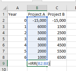
By using the “=IRR()” function we can confirm the IRR for project A and project B as 14.3% and 12.2% respectively – see if you can replicate these IRR solutions by downloading the file here: Example 2.5 & 2.6 data.
The Internal Rate of Return Decision Rule
As the internal rate of return occurs when the net present value is equal to zero, we can conclude that the IRR represents the highest rate of interest (cost of capital) an investor could afford to pay without losing money on a project if all funds were borrowed and the loan (principal and interest) were repaid (Bierman and Smidt, 2012). The IRR is therefore essentially a break even point for an investment after accounting for interest.
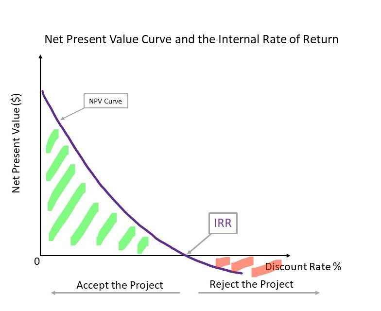
Consequently, once we know the IRR for a project, we can compare this IRR directly with the cost of borrowing at the prevailing market interest rate to finance the project, policy, or program. If we denote the cost of borrowing as r, the decision rule is:
- Accept the project if

- Reject the project if

The reason for this decision rule lies in the fact that companies, firms, and governments can often borrow at a lower interest rate to undertake the project and thereby experience the higher rate of return. Essentially, when calculating the internal rate of return we are effectively finding the annualised effective compounded rate of return. Therefore, in essence the IRR is capturing the opportunity for a profitable investment in a project, policy, or program.
Example 2.7
Suppose you calculated the IRR of the following project. Note: you can replicate this IRR result in Excel.
| Year | 0 | 1 | 2 | 3 | 4 | IRR |
|---|---|---|---|---|---|---|
| Project X | -5,000 | -1500 | 2000 | 3000 | 4000 | 11.6% |
- If the cost of borrowing to finance this project was 10% – the project should be accepted as IRR (11.6%) >
 (10%).
 - If the cost of borrowing was 12% – the project should be rejected as the IRR (11.6%) < (12%).
At this stage it is important to note that the IRR method will result in the same decision rule as the NPV method when we assume: (1) the projects are not mutually exclusive, and (2) there are no budgetary constraints that need to be considered. Under these conditions we would accept all projects where the .
For mutually exclusive projects, we should prioritise the project with the highest NPV. The reason for this is illustrated in the section on IRR limitations.[3]
The IRR and Hurdle Rates
A secondary decision rule may also be part of the acceptability of the project. Specifically, if the project investor has a required hurdle rate of return ( ), the project should be accepted if the
  and rejected if
  . This method is more appropriate when considering the CBA from an investor or private perspective where there is a company investing in the project, this is in comparison to the social cost-benefit analysis perspective we assume in this course.
Key Concept – Hurdle Rate
A Hurdle rate is the minimum rate that a company expects to earn when investing in a project. The hurdle rate is also often referred to as the company’s required rate of return, target rate, or minimum acceptable rate of return (MARR).
Example 2.8
Following from Example 2.7 above:
| Year | 0 | 1 | 2 | 3 | 4 | IRR |
|---|---|---|---|---|---|---|
| Project X | -5,000 | -1500 | 2000 | 3000 | 4000 | 11.6% |
If the company investing in this project requires all projects to have a minimum rate of return of 12.5% we would reject the project under the hurdle requirement as 11.6% < 12% required return for the company.
The Crossover Rate
One of the benefits of using the IRR to compare projects is it allows us to identify the exact crossover rate (also known as the switching rate). The crossover rate allows us to determine which project is preferred at various discount rates. It can be useful for comparing mutually exclusive projects at various discount rates. By taking the difference between the cashflows we can identify the discount rate where the preference between our projects switches using the incremental IRR.
Example 2.9
Again returning to Example 2.5. By taking the incremental difference between the net benefits of project A and project B and then calculating the incremental IRR on the difference we find the crossover rate of 9%. If project A and project B are mutually exclusive, project B is preferred to project A when the discount rate is less than 9%. For a discount rate above 9%, project A is preferred. At exactly 9%, we are indifferent between project A and project B.[4]
| Year | Project A | Project B | Difference (A) – (B) |
|---|---|---|---|
| 0 | -15,000 | -15,000 | 0 |
| 1 | 6000 | 1500 | 4,500 |
| 2 | 5000 | 2500 | 2,500 |
| 3 | 4000 | 3500 | 500 |
| 4 | 3000 | 4500 | -1,500 |
| 5 | 2000 | 5500 | -3,500 |
| 6 | 1000 | 6500 | -5,500 |
| IRR | 14.26% | 12.18% | 9.0% |
This result can also be identified in the graph as shown above in Figure 2.7 at the switching point.
Advantages of the IRR decision Rule
There are two clear advantages of using the IRR decision rule. Firstly, the IRR calculation does not rely on the selection of a discount rate. Secondly, for decision-makers the IRR is an easily understood criteria for decision-making providing an effective way to communicate the results to managers and professionals more broadly.
Limitations of IRR
There are quite a few limitations to using the internal rate of return decision rule as the core decision rule when evaluating policies, programs, or projects.
IRR Comparison to the Status Quo
Using the IRR as a measure of the net social benefit is only considered appropriate if there is only one alternative project that is being compared to the status quo or the projects are not mutually exclusive. In this instance where we are comparing a single policy or project to the status quo, the result from the IRR decision rule will be the same as the NPV decision rule. Specifically:
- If the IRR is greater than the discount rate (
 ), then it follows that the NPV would be greater than zero at the same discount rate (
 at ) – therefore both the IRR decision rule and the NPV decision rule would lead you to accept the project.
 - If the IRR is less than the discount rate (
 ), then it follows that the NPV would be less than zero at the same discount rate (
 at ) – therefore both the IRR decision rule and the NPV decision rule would lead you to reject the project.
This can be seen clearly in our NPV curve Figure 2.9.
However as mentioned above when we discussed hurdle rates, the IRR can be used as a threshold requirement for private CBAs i.e., an investment project should be undertaken if the IRR is greater than a required rate of return, usually set as a company or department standard rate of return. In these instances where a hurdle rate is required using the IRR decision rule may not result in the same conclusion as the NPV decision rule.
Multiple IRRs and No IRRs
One significant limitation of using the internal rate of return to drive the decision to accept or reject a project is caused by the potential for multiple or indeterminant IRRs. This often occurs when there is an stream of unconventional cash flows or net benefits. An unconventional net benefit stream is when there is a series of inflows and outflows that change the sign of the net benefit more than once. This usually occurs when the stream of net benefits follows an unconventional format due to high future costs. This is in comparison to a conventional net benefit stream where the sign changes only once (i.e., an initial cost, followed by a series of positive net benefits).[5]
If one of future net benefit streams of a project changes sign, there will be multiple internal rates of return. For example, if the net benefit of a conventional stream follows a – , +, -, + format, the switching of the sign creates an unconventional net benefit stream.
Example 2.10
Consider a project with the following net benefits:
| Year | 0 | 1 | 2 |
|---|---|---|---|
| Net Benefit | -200 | 460 | -264 |
As seen from the table above, the net benefit is unconventional following a – , + , – format where we observe later benefit streams experience a sign switch in comparison to the conventional – , +, + format.
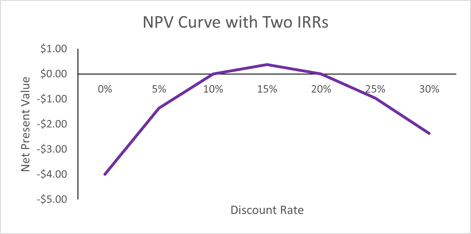
When plotting the NPV curve for this project, we can see that the curve intersects the x-axis twice indicating that there are two points on the curve where the NPV is zero at 10% and 20%. See if you can replicate this NPV curve by downloading this file: Example 2.10
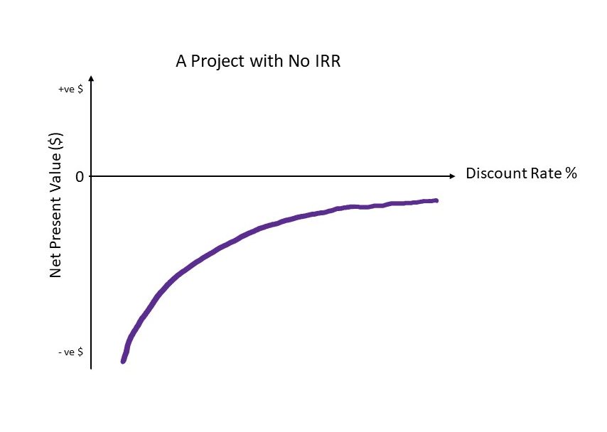
As seen in Example 2.10, it is possible to have more than one internal rate of return which results in difficulties in identifying the correct internal rate of return for a project. There can also be situations where there is no internal rate of return. This occurs when there is no change in the sign of the net benefit stream – and therefore there is no discount rate that would produce a NPV of zero. This occurs often in healthcare projects which often only run at a cost to a government. The NPV curve of such a project would look similar to Figure 2.11.
IRR and the Scale of a Policy or Project
The IRR also does not necessarily consider the scale or the size of the project under consideration.
Example 2.11
If we have two projects that are mutually exclusive. Project A has an initial cost of $200 and project B has a cost of $10. If the life of the projects is two years and the benefits are summarised in Table 2.12. The IRR can be calculated as:
| Year | 0 | 1 | 2 | IRR | NPV @ 5% DR |
|---|---|---|---|---|---|
| NPV A | -200 | 120 | 120 | 13% | $ 23.13 |
| NPV B | -10 | 7 | 7 | 26% | $ 3.02 |
In this instance if we made a decision to accept the highest IRR project, we would potentially select the project with a smaller net present value. For example, if the appropriate discount rate is 5% using the IRR decision rule, we would select project B. However, project A clearly has a higher NPV and should be selected over project B.
NPV vs IRR Decision Rule
As a consequence of the limitations of the IRR, it is clear that we should give preference to the NPV decision rule when comparing multiple projects in the case where the projects are mutually exclusive. This is because the NPV will lead to the maximisation of net benefits. The NPV rule will lead to a clearer evaluation on which project provides the largest net benefit – thereby achieving allocative efficiency.
Benefit-Cost Ratio
The final indicator that we use for the evaluation of the net social benefit of a policy, program, or project is the benefit-cost ratio (BCR). The purpose of the benefit-cost ratio is to show the ratio of the present value of the benefits to the present value of the costs instead of showing the net present value in absolute terms. Consequently, the higher the ratio the more attractive the project is. Overall, the BCR attempts to summarise the overall value for money in a project. We calculate the BCR using the following formula:
(11) 
The BCR therefore expresses the proportion of benefits to costs.
Benefit-Cost Ratio Decision Rule
The BCR is simply another way of expressing the NPV decision rule in a more intuitive method. If the present value of benefits are greater than the present value of costs, then we know that the NPV is positive. This is equivalent to:
(12) 
We know that:
(13) 
Hence, the decision rule for the BCR is to accept the project if the discounted benefits divided by the discounted costs (initial capital and ongoing costs) is greater or equal to 1. i.e.,
(14) 
Following from this definition, we can highlight these results:
1) If the  we should reject the project as the NPV would be negative. This also implies that the IRR of the project in question is less than the discount rate.
2) If the  we are indifferent between accepting or rejecting the project as the NPV would be equal to zero and the IRR is equal to the discount rate.
3) If the  we should accept the project as the NPV would be positive. This also implies that the IRR of the project is greater than the discount rate.
Overall this implies that when considering a project relative to the status quo, we accept the project if the  . We reject a project if the . When comparing projects that are not mutually exclusive, we should accept all projects if the , assuming there are no budgetary constraints. However, we should abstain from using the BCR when considering mutually exclusive projects or where there are budgetary constraints.
Advantages of the Benefit-Cost Ratio
The advantage of the benefit-cost ratio is it indicates the value the policy, program, or project generates per dollar in costs. The BCR also accounts for the time value of money as it uses the discounted benefits and costs in the calculation.
Limitations of the Benefit-Cost Ratio
The BCR method provides no additional information that was not already provided by the NPV method. However, when using the BCR we lose information relating to the magnitude of the project. For example, if we are considering two projects as follows:
- Project A: PV(Benefits) = $10,000 and PV(Costs) = $2,000. Therefore, the BCR = $10,000/ $2,000 = 5
- Project B: PV(Benefits) = $500 and PV(Costs) = $1,00. Therefore, the BCR = $5,00/ $100 = 5
Secondly, the benefit-cost ratio can result in the incorrect ranking of mutually exclusive projects. Therefore, we can use the BCR to evaluate the efficacy of a single project, but it should not be used to rank projects as it may result in the acceptance of projects that are not as allocative efficient as the best choice from the NPV method.
Example 2.12
Suppose we are considering the following mutually exclusive projects which are within our budget. Assume that Project A and Project B follow a conventional net benefit stream where there is an initial cost in year 0 and benefits accrued across years 1-5.
| Year | 0 | 1 | 2 | 3 | 4 | 5 |
|---|---|---|---|---|---|---|
| Project A | -1000 | 300 | 300 | 300 | 300 | 300 |
| Project B | -2000 | 550 | 550 | 550 | 550 | 550 |
If the appropriate discount rate is 5%. We can calculate the NPV of both Project A and Project B
Calculating the NPV of Project A:

Calculating the NPV of Project B:

Based on the NPV decision rule  . therefore we would accept project B. However, if we look at the BCR we see a different story:

and

Example 2.12 shows that in the instance where the BCR was the only information we have for our decision-making, we would be making the wrong project choice which would lead to an inefficient allocation of our available resources. This BCR result is therefore misleading. Consequently we should always use the NPV for ranking decisions.
NPV vs BCR Decision Rule
As a consequence of the limitations of the BCR, it is clear that we should preference the NPV decision rule when comparing multiple projects in the case where the projects are mutually exclusive. Again, this is because the NPV decision will lead to the maximisation of the net benefit which is therefore more allocatively efficient.
EXCEL Skills
If you have never used excel before, please refer to this Youtube video by GCFLearn.org that explains how to open Excel and get started with the available ribbon tabs.
Revision
Summary of Learning Objectives
- Projects, programs, or policies can have short-term impacts or long-term impacts. Discounting allows an analyst to account for the period of time for which the benefits and costs accrue.
- The present value of a project can be discounted over a single period or multiple periods. Future values can be compounded over a single period or multiple periods where appropriate.
- There are three key methods for evaluating the net social benefit: (1) the Net Present Value, (2) the Internal Rate of Return and the (3) Benefit-Cost Ratio.
- The NPV decision rule is preferred in cost-benefit analysis.
References
Stokey, E., & Zeckhauser, R. (1978). A primer for policy analysis. W. W. Norton.
Bierman, J. R., & Smidt, S. (2012). The capital budgeting decision: economic analysis of investment projects. Routledge.
- Net benefit is the term used here as there are no social impacts of the investment that need to be accounted for. ↵
- Similar to how a decision rule is formulated in your introductory statistics course. The decision rule identifies the circumstances where you reject or do not reject the null hypothesis under investigation. However, in the instance of decision rules in CBA we are creating a clearly defined rule where we reject or do not reject the project under consideration relative to the status quo or base case scenario. ↵
- If we selected the project with the highest IRR we can accidentally select a project with a lower NPV. This is a problem when projects are mutually exclusive as we should always choose the project with the highest NPV when projects are mutually exclusive to ensure we achieve allocative efficiency. ↵
- Note that the NPV A is approximately $2 higher than NPV B at 9%. Consequently, at 9% we should select project A. ↵
- Projects, programs, or policies with unconventional cashflows have other issues that may affect their attractiveness. ↵
