
Chapter 10: Dealing With Uncertainty
Learning Objectives
After completing this chapter, students should be able to:
-
Identify and address uncertainty to estimate the net social benefit in a cost-benefit analysis.
-
Identify and evaluate risk in a cost-benefit analysis including expected value analysis.
-
Understand risk preferences in the context of cost-benefit analysis.
-
Implement sensitivity analysis in Microsoft Excel.
-
Effectively communicate the results of a sensitivity analysis.
Dealing with Uncertainty and Sensitivity Analysis – How Big is a Piece of String?
Up until this point, we have assumed that all costs and benefits were known with certainty – however this is not a valid assumption. When conducting a cost-benefit analysis (CBA), an analyst often relies on estimates for variables that cannot be predicted with complete accuracy. Consequently, the result of the CBA is subject to risk and uncertainty, as the result cannot be determined with complete confidence. This chapter focuses on how a CBA analyst can evaluate risk and uncertainty involved in implementing a policy, program, or project to ensure the final recommendations provide clear decisions.
It is important to note that there is no exact method for dealing with uncertainty. However, it is important for an analyst to evaluate how risk and uncertainty may impact the result of the CBA. Despite this limitation, uncertainty must be evaluated in some form to determine if the results of the CBA are robust and consistent.
Risk Versus Uncertainty
Risk is when the probability of the potential outcomes are known. When we can assign probabilities to all possible outcomes, and the set of possible outcomes is known the level of risk can be evaluated. Risk is often expressed as the expected outcome given the information available to the analyst. It is possible to quantify and evaluated risk using models. An example of risk would be placing a gamble on rolling a 1 when rolling a single die (1 in 6 chance) or when flipping a coin there is a 50 percent probability of “heads”. Under these circumstances, we can evaluate the risk as the outcome set is known along with the associated probabilities of each outcome.
Uncertainty is when the probability of outcomes is unknown or cannot be reasonably identified. We do not know all the possible outcomes and cannot assign probabilities to the outcomes. In addition to this, it is not possible for an analyst to control the level of uncertainty. An example of uncertainty is when we cannot predict when the next pandemic or epidemic. When the COVID-19 pandemic began, the likelihood of getting sick was unknown and the probability of dying was unknown – therefore it falls under uncertainty.
Key Concept – Risk vs Uncertainty
Risk is where the probabilities of potential outcomes are known, while uncertainty involves unknown probabilities and unknown outcomes.
Risk
Risk can be subjective or objective. Subjective risk is an individual’s perception of the likelihood of an event based their opinion. Subjective risk can be different for each individual assessing and evaluating a situation or series of outcomes. Risk perceptions and heuristics can create bias in the evaluation of subjective risk such as optimism bias.[1]
Objective risk involves deduction from previous occurrences of an event. Therefore, we can describe objective risk based on actual variations in outcomes. For example, there is a 50% chance when you toss a coin it is “heads” or a 1 in 6 chance that when you roll a dice you get a 3. It is possible to calculate objective risk by identifying the difference between the actual outcome and the expected outcome in an ex-post CBA.
Consequently, objective risk in CBA usually uses historical information whereas subjective risk in CBA relates to values assigned by the CBA analyst. Subjective risk differs from objective risk as the person identifying the risk or probability of an event has no way of identifying the actual likelihood of an event happening. In most cases, cost-benefit analysis involves some level of subjective judgement relating to the probabilities of potential outcomes. For example, cost-benefit analysis often relies on estimates of willingness-to-pay which captures subjective evaluations. Therefore, measures of willingness-to-pay are susceptible to subjective risk.
Distinguishing between the types of risk helps analysts better understand how risk will affect decision-making. It is well known that objective risk is observable and can be calculated using data and statistical information providing improved confidence in the results. However, in many instances in CBA the policies or projects may not be repeated and therefore the historical information may not be available for the evaluation of objective risk (i.e., there is no data available to assist the decision-making process).
Subjective risk has an element of psychological uncertainty as it is based on personal experience or perceptions. Additionally, subjective risk is known to alter the behaviour of people. For example, when people take out car insurance they engage in more risky driving behaviours (moral hazard). However, the use of subjective risk evaluation is to ensure consistency in decision-making across all information known to the analyst, taking a more holistic approach to the evaluation of risk.
Uncertainty
Uncertainty is a concern for all decision-makers. As part of the evaluation of a policy or program, uncertainties should be identified, and evaluated in a way that improves understanding of the policy or project under consideration. Values inputted into a cost-benefit analysis are forecasts of future impacts. Uncertainty arises from the possibility that the forecasts will be incorrect. Therefore, forecasts in cost-benefit analysis are tied to uncertainty. It is impossible for an analyst to identify all factors that may impact the net social benefit of a project under consideration. But, it is important to evaluate those uncertainties that matter most.
Uncertainty can be internal or external to the project (endogenous or exogenous respectively). When uncertainty is internal to the project, there is an element of control over the input. Alternatively, external uncertainty comes from those factors beyond the control of the project. It is important to differentiate between the two types of uncertainty – those we can control and those we cannot – as the implications for the analysis differ. Consider a project for the development of a solar power station. The external uncertainty would relate to the market competition for electricity and internal uncertainty would be the price charged by the company for the electricity.
Furthermore, in CBA it is common practice to treat expected values as certain. Specifically, we have assumed constant year 0 pricing (real pricing) where the price does not change over time which required the use of the real discount rate. This involved inputting values used in the CBA as point estimates within the spreadsheet. However, it is likely that prices will change over time. Projects or polies with long durations will have uncertainty around the values. Consequently, an analyst should not pretend that the results are precise as their results represent only the best guess.
Key Concept – Point Estimate.
A point estimate is a single value which is a “best guess” or “best estimate” of the value. So far in CBA, we have assumed the NPV result is certain and represents a point estimate of the project.
Additionally, an analyst cannot identify all factors that may impact the profitability of a policy or project, but it is important to identify the inputs which may change. Keep in mind that if the point estimates used in the CBA are inappropriate, then the resulting CBA is pointless. This comes down to the concept of “garbage in – garbage out”. The idea of garbage in – garbage out originated from computer science and information technology. The idea is that poorer quality information will result in poorer quality analysis of uncertainty. Although uncertainty does not mean that the input data is inaccurate, an analyst needs to be aware of this issue.

Overall, when evaluating risk and uncertainty in CBA it is important to evaluate: (1) what the degree of uncertainty is, (2) whether the uncertainty is a significant risk, and (3) whether the risk is acceptable. By doing this, we can ensure the processes used to evaluate the NPV of a project is robust as possible.
Expected Value Analysis
Expected value analysis can be conducted if the possible set of outcomes can be defined. Expected value analysis involves modelling uncertainty as a set of contingencies with specified probabilities of occurrence. To model risk using expected value analysis, we need to know the set of possible outcomes (or potential “states of the world” in the future) and the probability of observing each of the possible outcomes.
This set of contingencies or events needs to be mutually exclusive and collectively exhaustive. Mutually exclusive implies that only one future state of the world can be observed. Collectively exhaustive means within the set of events, one of the events must occur in the future (i.e., one outcome of the set of potential outcomes is observed in the future). This directly relates to the rules of probability such that:
(1) The probability of a random event ( ) lies between 0% and 100% chance for any event

for all and
(2) the total sum of probabilities is equal to 1

for all .
To calculate the expected value, we multiply each possible outcome by the probability of observing that outcome:
![\begin{equation*} E[X] = \sum X_i. p_i(X_i) \end{equation*}](https://uq.pressbooks.pub/app/uploads/quicklatex/quicklatex.com-07c7b0045751f40ec6258539cf3d36e6_l3.png "Rendered by QuickLaTeX.com")
where is the event or outcome and  is the probability of observing that event. These two probability conditions must be met to calculate the expected value.
If we know the set of possible “states of the world” we could face in the future, we can calculate the expected net present value (or expected net benefit) as follows:
(1) ![\begin{equation*} E[NPV] = \sum (p_i \times NPV_i) \end{equation*}](https://uq.pressbooks.pub/app/uploads/quicklatex/quicklatex.com-e6086b6caa39321734d19955cfab09f8_l3.png "Rendered by QuickLaTeX.com")
where  is the NPV in state of the world
  and is the associated probability. Consequently, the expected NPV is the average of the possible outcomes from the project weighted by their probabilities. Hence, the expected NPV indicates the average outcome of the risky decision, if the decision were repeated a large number of times. If the expected NPV is positive, it suggests that the project should be undertaken. This is often referred to as the expected NPV decision rule.
Note that if a decision-maker has imperfect knowledge about the outcome of a project there is still a risk associated with that project – even if the expected NPV is positive. If potential NPVs are below zero, it is possible to experience a negative NPV after implementing the project. However, under the NPV decision rule with certainty a project would be rejected if the NPV was negative. In expected value analysis, if one or more of the possible NPV outcomes is negative, it is crucial to consider further evaluation of potential outcomes using simulation such as Monte Carlo to reduce uncertainty and make a more informed decision.
Additionally, the expected NPV decision rule requires the decision-maker to be risk neutral. A decision-maker is considered risk neutral if the decision-maker is indifferent between an expected value of $X and $X with certainty. Treating expected values as if they are certain implies we are risk neutral – indifferent between certainty and the risky gable outlined in the section below on Risk Neutrality. In reality, decision-makers are not necessarily risk neutral. If the decision-maker is risk averse it would be inappropriate to use the expected NPV decision rule.
Example 10.1
Example – Calculating Expected NPV
Suppose there are three possible outcomes – a high NPV estimate of $40,000, a best guess estimate at $35,000 and a low NPV estimate of $10,000. The associated probabilities of each possible outcome of the project are summarised in Table 10.1
| Scenario | Probability | NPV (Xi) | Prob x NPV(Xi) |
|---|---|---|---|
| High | 0.2 | 40,000 | 8,000 |
| Best Guess | 0.4 | 35,000 | 14,000 |
| Low | 0.4 | 10,000 | 4,000 |
![E[NPV] =](https://uq.pressbooks.pub/app/uploads/quicklatex/quicklatex.com-cf7015735565f9032c54e2169add15e5_l3.png "Rendered by QuickLaTeX.com")

 probability of +
 probability of +
  probability of
 +
+  +
+
$8,000 + $14,000 + $4,000
$26,000
To calculate this example in Excel you can download the spreadsheet here: Example 10_1
You can download the spreadsheet for the above H5P question here: Exercise 10_1
One limitation of expected value analysis is the dispersion of potential outcomes is not captured. The expected value only provides information on the Expected NPV. It does not capture the dispersion of potential NPV outcomes. The dispersion (also known as the spread) of outcomes captures the risk of the project. Consequently, to measure the absolute measure of risk we calculate the standard deviation of the project.
To calculate the standard deviation, we need to calculate the variance. The formula for variance is:
(2) ![\begin{equation*} \sigma^2_{NPV} = \sum_{i=1}^{n} p_i.(NPV_i - E[NPV])^2 \end{equation*}](https://uq.pressbooks.pub/app/uploads/quicklatex/quicklatex.com-8af52070b66511ed915795c0372ce314_l3.png "Rendered by QuickLaTeX.com")
Variance is a measure of risk – the higher the variance, the greater the risks associated with the probability distribution. However, standard deviation is the preferred metric of risk. This is because variance is measured in squared units. The standard deviation removes this aspect. Taking the square root of the variance gives the standard deviation i.e., ![\sigma[NPV] = \sqrt(\sigma^2[NPV])](https://uq.pressbooks.pub/app/uploads/quicklatex/quicklatex.com-07139571d980f75c6a76c16cd8090ba1_l3.png "Rendered by QuickLaTeX.com") . The higher the standard deviation the greater the risk. The standard deviation provides information in the spread of NPV outcomes relative to the expected value. The larger the standard deviation, the more risk is involved in the project. Similarly, the smaller the standard deviation the lower the risk.
. The higher the standard deviation the greater the risk. The standard deviation provides information in the spread of NPV outcomes relative to the expected value. The larger the standard deviation, the more risk is involved in the project. Similarly, the smaller the standard deviation the lower the risk.
Example 10.2
Example – Calculating Variance and Standard Deviation of NPV
Consider the information from Example 10.1, replicated in the table below:
| Scenario | Probability | NPV (Xi) | NPV(Xi) – E(NPV) |
|---|---|---|---|
| High | 0.2 | 40,000 | 14,000 |
| Best Guess | 0.4 | 35,000 | 9,000 |
| Low | 0.4 | 10,000 | -16,000 |
| Expected Value | 26,000 |
From this example we can see the favourable outcome (high) has a probability of 20%, the best guess outcome has a probability of 40% and the unfavourable outcome (low) has a probability of 40%. These probabilities indicate that there is a high likelihood of an outcome of $35,000 or below (an 80% chance).
Using Table 10.3, we can understand how to effectively apply the variance formula. First, we calculate the expected NPV (column 2) by taking the sum of probability weighted outcomes. Then we take the difference between each potential NPV outcome and the expected NPV (column 3). The difference is then squared (column 4). Finally, each of the squared differences is multiplied by the associated probability (column 4 multiplied by column 1). This result is then summed for the variance.

 –
– ![E(NPV)]^2](https://uq.pressbooks.pub/app/uploads/quicklatex/quicklatex.com-a315cd5a0300af04b9fdbdc08b4d857d_l3.png "Rendered by QuickLaTeX.com")

To subsequently find the standard deviation which represents the risk in outcomes, we take the square root of the variance i.e.,  . To calculate it using the formula by hand:
![\begin{align*} \sigma^2_{NPV} &= \sum_{i=1}^{n} p_i.(NPV_i - E[NPV])^2 \\ & = 0.2 \times (40,000 - 26,000)^2 + 0.4 \times (35,000 - 26,000)^2 \\ & + 0.4 \times (10,000 - 26,000)^2 \\ & = 174,000,000 \end{align*}](https://uq.pressbooks.pub/app/uploads/quicklatex/quicklatex.com-50b71a56d8b3e533eedd9d0a244d1617_l3.png "Rendered by QuickLaTeX.com")
To replicate this example you can download the spreadsheet here: Example10_2
Standard deviation is usually used to measure risk instead of variance as the interpretation of standard deviation is more intuitive with respect to the unit of measure. Variance for the NPV of a project will be measured in squared dollars ($ ), whereas standard deviation is measured in dollars ($).
Discrete vs Continuous Probability
There are many ways we can model risk in a cost-benefit analysis. Rather than using a point estimate (a single value) for an input in a CBA, it is possible to utilise discrete or continuous probability distributions to account for risk. The examples above use discrete probability to evaluate the risk associated with a policy or project. By modelling on a set of potential possible input values, uncertainty can be reduced. Computer programs such as the @risk add-in for Excel can be used when inputs are subject to continuous probability distributions.
Types of Uncertainty in CBA
We can categorise uncertainty into two types in CBA:
1) Uncertainty faced by economic agents – reflected in the approximation of willingness-to-pay and social surpluses (consumer and producer surpluses).
2) Uncertainty faced by the CBA analyst or policymaker – relating to the selection of inputs into the framework for analysis.
Uncertainty Faced by Economic Agents – Risk Aversion
In economics and finance, attitudes to risk matter. We can categorise economic agent or individual into one of three possible categories: Risk averse, risk neutral, and risk loving.
Suppose we consider comparing $100,000 with certainty against a gamble – the gamble has a 50% chance of giving 50,000 and 50% chance of $150,000. The expected value of the gamble is $100,000.
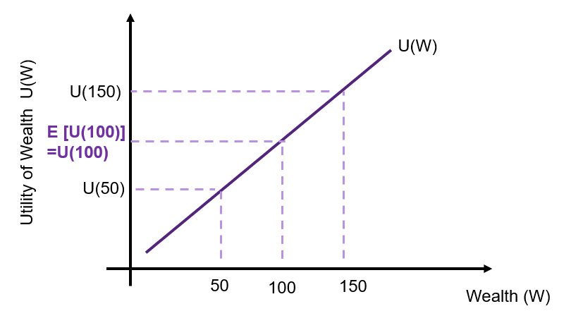
Risk Neutral
A risk neutral individual is indifferent between a risky gamble and the payoff with certainty. This is illustrated in Figure 10.2 where the x-axis represents an individual’s wealth, and the y-axis represents the utility derived from the wealth received. There is a linear relationship between wealth and utility. The utility is equal between the $100,000 with certainty and the risky gamble with the expected payoff of $100,000 i.e., ![E[U(100)] = U(100)](https://uq.pressbooks.pub/app/uploads/quicklatex/quicklatex.com-87b4b17a80609fd302efb355408831fe_l3.png "Rendered by QuickLaTeX.com") .
.
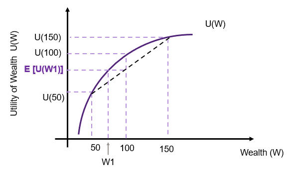
Risk Averse
A risk averse individual has diminishing marginal utility (increasing utility at a decreasing rate) as shown in Figure 10.3. Again, consider the risky gamble relative to the $100,000 with certainty.
The black dashed line represents the utility from the gamble – given as the tangent between the $50,000 and the $150,000. In this instance, a risk averse individual prefers $100,000 with certainty over the gamble. The utility from the certain $100,000 is  and it is above the expected utility received from the risky gamble
 ![E[U(W1)]](https://uq.pressbooks.pub/app/uploads/quicklatex/quicklatex.com-cdce623ae19e3400545cb9b267612933_l3.png "Rendered by QuickLaTeX.com") . is known as the certainty equivalent. The difference between 100 and W1 is the risk premium. The price the individual is willing to pay to ensure they receive
. is known as the certainty equivalent. The difference between 100 and W1 is the risk premium. The price the individual is willing to pay to ensure they receive  with certainty in the gamble.
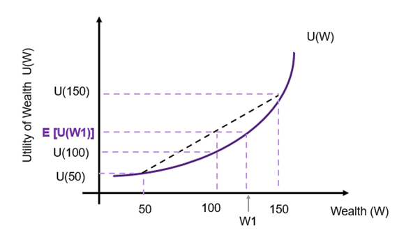
Risk Seeking
A risk seeking individual has an increase marginal utility (increasing at an increasing rate) as shown in Figure 10.4. Again, the black dashed line represents the utility from the gamble – given as the tangent between the $50,000 and the $150,000. In this instance, the individual prefers the risky gamble to the certainty of $100,000. This is shown through ![E[U(W1)] > U(100)](https://uq.pressbooks.pub/app/uploads/quicklatex/quicklatex.com-2a466b126e3f21330f51631e8468cdd3_l3.png "Rendered by QuickLaTeX.com") . As a risk seeker, the individual would be willing to pay the difference between 100 and W1 to take the risk.
. As a risk seeker, the individual would be willing to pay the difference between 100 and W1 to take the risk.
By better understanding the risk profiles of individuals, we can account for risk aversion in our cost-benefit analysis. An example of the application of risk aversion to cost-benefit analysis can be found in this paper by Kind, Wouter Botzen and Aerts (2016).
Uncertainty Faced by the CBA Analyst or Policymaker
This type of uncertainty relates to the lack of information around the point estimates used in the CBA. To deal with uncertainty faced by the CBA analyst or policymaker, we implement sensitivity analysis outlined in the section below on Sensitivity Analysis .
At this stage, it is important to note that when assessing a policy or project from the viewpoint of the government sector, an analyst often assumes a risk neutral profile. This is based on the aggregation of preference across stakeholders. However, it is possible to consider other risk profiles.
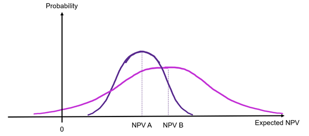
Projects with Different Degrees of Risk
The expected net benefit or expected net present value does not highlight which project to select based in individual risk preferences. Choice of projects depends on a decision-maker’s attitude to risk.
If we consider two projects (A and B) with different standard deviations as illustrated in Figure 10.5. As can be seen, if we evaluate the decision purely on the NPV, project B would be selected as  . However, evaluating the decision purely based on the NPV does not account for the fact that project B has a higher variation than project A i.e., project B is more dispersed and project A’s NPV can be considered more certain. Consequently, the decision on whether the decision-maker is risk averse or a risk taker.
To determine selection of projects based on risk preferences, we need to calculate the standard deviation. Using the information of both the risk and the expected NPV it is possible to evaluate the choice of project under different risk profiles. A risk neutral investor will prefer the project with the highest expected NPV. A risk seeker is willing to take on more risk (a higher standard deviation) for a greater reward, seeking a project with a higher risk if it provides a higher return. In this instance a risk seeker will likely take on a project with a higher level of risk if it is associated with a higher return. A risk averse individual would consider the trade-off between the expected NPV and the dispersion of possible NPV outcomes.[2]
Sensitivity Analysis
Sensitivity analysis is a straightforward way to address uncertainty in cost-benefit analysis. Sensitivity analysis involves the evaluation of which outcomes are sensitive to the assumed inputs in the cost-benefit analysis. In this instance the outcomes we are evaluating are the net present value (NPV), internal rate of return (IRR), and the benefit-cost ratio (BCR). The purpose of a sensitivity analysis is to determine how much the net social benefit changes when assumed input values change. Sensitivity analysis is crucial as it identifies how independent inputs into the policy, program, or project can impact on the net present value – and therefore the potential profitability or desirability of the project.
Any cost-benefit analysis should be subject to a sensitivity analysis. Consequently, the sensitivity analysis is the last major step of the CBA before providing the recommendation or action.[3] Key components of the project should be subject to sensitivity analysis. If the net social benefit does not change significantly after the completion of a sensitivity analysis, the result of the CBA can be considered robust. Keep in mind that evaluating potential outcomes under uncertainty is a subjective assessment and the selection of inputs for evaluation as part of the sensitivity analysis is also subjective.
The process of implementing a sensitivity analysis involves changing the underlying inputs that are key to the project to alternative potential assumptions to identify the impact of that variable (such as labour costs, initial capital costs, cost of resources, tax rates, et cetera.). This can involve changes in input prices or input quantities. There are four key reasons for conducting a sensitivity analysis:
1) Improves the robustness of the CBA results.
2) Allows for better understanding of the project and communication of results.
3) Reduce uncertainties through identification of inputs that cause significant fluctuations in the outcomes of interest. i.e., which factors will significantly affect the NPV of a project.
4) Provides an opportunity assess and effectively understand risks associated with a policy, project, or program.
We cannot use sensitivity analysis to predict the likelihood of an outcome, but we can check the extent to which the outcome is robust to a change in an estimated input used as part of the prediction and monetisation process. If the impact of a change in an input subject to sensitivity analysis is sufficiently large in percentage terms, the robustness of the CBA can be called into question.
Sensitivity Analysis and the Discount Rate
The discount rate must always be subject to a sensitivity analysis. Specifically, in the implementation of policies or projects, the forecasts used will be sensitive to a change in the discount rate. In most instances, government departments have a range of discount rates that must be used in a CBA. However, in some instances it may be difficult to determine the appropriate discount rate. For example, the choice of discount rate for climate change mitigation is subject to much discussion and there is no set discount rate choice.
An analyst must evaluate the impact of the discount rate on the NPV of a project for several reasons:
- There is a clear inverse relationship between the NPV and the discount rate – as the discount rate increases, the NPV decreases. This was observed when we plotted NPV curves in the past.
- Selecting the wrong discount rate can potentially change the decision to accept or reject a project.
- When a project incurs large costs early and benefits later are more susceptible to changes in the discount rate. The choice of discount rate can make the NPV more susceptible to fluctuations.
Evaluating the choice of discount rate improves the robustness of the CBA. If the NPV is greater than zero under all discount rates considered as part of the sensitivity analysis, the results can be considered sufficient to support acceptance of the project. In the past we have implicitly completed a sensitivity analysis of the discount rate by looking at how a change in the discount rate impacts the NPV.[4] It is possible to use any range for the sensitivity analysis on the discount rate.
We can also utilise the IRR to understand how sensitive a project is to the discount rate. As mentioned before, plotting the NPV curve identifies the IRR when the curve intersects the x-axis (Figure 2.6 from Chapter 2). This point is where the NPV is equal to zero, hence if the IRR is equal to the discount rate, the projects NPV would be zero and a risk neutral decision-maker would be indifferent between accepting and rejecting the project. If the IRR is higher than the discount rate, then it provides an economic justification to undertake the project. It is important to note that a high IRR may suggest a project is less sensitive to changes in the project inputs.
Example 10.3
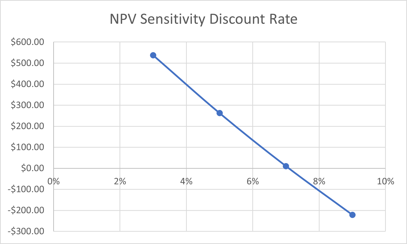
A project has the following costs and benefits over the life of the project summarised in Table 10.4. The results for a sensitivity analysis using 3, 5, 7 and 9% as the discount rate for the project is shown at the bottom of the table. The NPVs were calculated using the =NPV() function covered in Chapters 2 and 3.
The results of the sensitivity analysis can easily be summarised in a graphical illustration as shown in Figure 10.5 below. This is the NPV curve, plotted using the selected range of discount rates used in the sensitivity analysis.
To replicate this example, you can download the spreadsheet here: Example10_3
Other Factors to Consider in a Sensitivity Analysis
A sensitivity analysis should be conducted on any project input that may be expected to have a significant impact on the outcome of the project (as measured by the NPV, IRR, or BCR). It is often suggested that an analyst considers conducting a sensitivity analysis in inputs such as:
– horizon/salvage values
– wages
– the value of statistical life
– environmental impacts
– growth rates
– revenues (including price and quantity produced)
This list is not exhaustive but provides a starting point for evaluating which inputs to consider when conducting the sensitivity analysis. One way of determining which cost or benefit inputs should be evaluated as part of the sensitivity analysis is by varying each input, holding all other inputs constant and observing the change in the NPV.[5] Those factors that change the NPV significantly or change the sign of the NPV should be investigated further as part of the sensitivity analysis.
Additionally, when a point estimate is calculated as an input to the project (such as calculating a non-market shadow price), the confidence interval from the estimation process will provide an idea of how sensitive the project is to the point estimate element.
Types of Sensitivity Analysis
We will look at three types of sensitivity analysis:
1) Partial sensitivity analysis
– Single variable (One Factor)
– Two Factor (using “What-if Analysis?” in Excel)
2) Best-worst case scenario analysis
3) Simulation (such as Monte Carlo)
The choices of which sensitivity analysis to utilise depends on the context of the project and the type of risk involved
Partial Sensitivity Analysis
Partial sensitivity analysis is the most commonly used approach to assess the sensitivity of the NPV to a change in an assumed value for an input. A partial sensitivity analysis involves changing only one input or factor used in the CBA at a time. Example 10.3 above where only the discount rate was changed is an example of a partial sensitivity analysis.
To complete a partial sensitivity analysis in Excel, create a column or row of values you wish to consider. Then change the relevant cell to the values you have specified to compute the new NPV, BCR, or IRR. You can then record the results in Excel. This information can then be used to visualise the results of the partial sensitivity analysis.
Example 10.4
Example – Single Variable Sensitivity Analysis (One Way Partial Sensitivity)
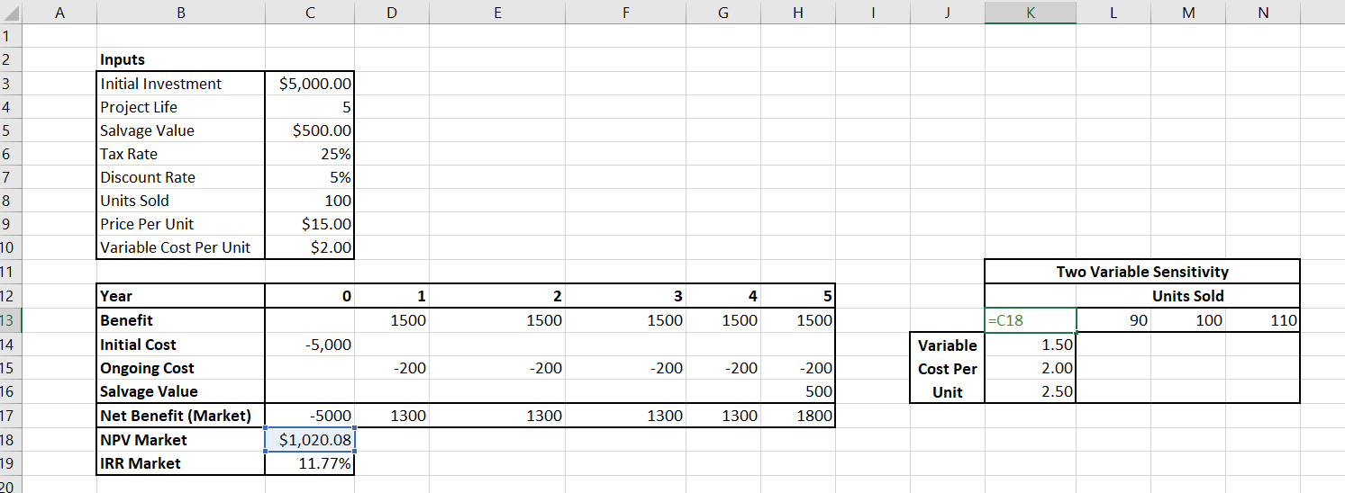
Suppose a company is considering a project that will produce 100 widgets per year, over 5 years. The initial cost of the project is expected to be $5,000. To produce the widgets there is a variable cost of $2.00 per widget. Each widget is expected to be sold for $15.00. The company tax rate is 25% and after the project is finished, the salvage value would be $500. This information is summarised in Table 10.5.
Inputs:
If the appropriate discount rate is 5%, it is possible to calculate the market perspective as shown in Table 10.6 below:
To conduct a partial sensitivity analysis, we change only one input – holding all other inputs constant. This involves changing only one cell to see how the NPV and the IRR change. For example, we can change the discount rate by 1% increments between the range of 3% to 7%. The NPV at 3% would be $1,384.92, at 4% $1,198.33 etc. It is possible to conduct a partial sensitivity analysis on many other inputs into this CBA. An example summary of a partial sensitivity analysis is provided below in Table 10.7.
See if you can replicate this table by downloading the spreadsheet here: Example10_4
After a partial sensitivity analysis has been conducted it is possible to identify the key variables that impact the NPV significantly. From this point it is possible to generate a table of results that allow for variations in combination for the inputs. This is illustrated in the two variable partial sensitivity analysis outlined in Example 10.5 below.
Example 10.5
Example – Two Variable Partial Sensitivity Analysis
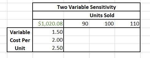
Consider the company from Example 10.4 above. We have the following information on the best guess (point estimates) for the project summarised in Table 10.8.
We can use the “What If Analysis” function in Excel to conduct a two variable partial sensitivity analysis. Suppose the company is interested in conducting an analysis on the number of widgets sold varying by -/+10%, and the variable cost per unit, varying by -/+25%. To conduct an analysis of changes in these two inputs we need to create a matrix table as shown in Figure 10.6, where the Units Sold has been provided in the row and the variable cost per unit is in the column of the matrix.
The information in the top left references the output we wish to conduct the sensitivity analysis on – in this case the Net Present Value from our best guess estimate of the CBA. We must equate this cell to the output from the market analysis as shown in Figure 10.7 below.
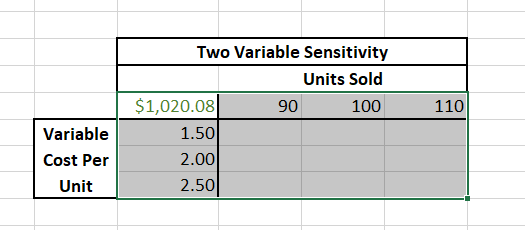
Once we have referenced the output cell for the sensitivity analysis, we have to highlight the matrix including the rows and columns as shown in Figure 10.8.
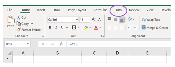
Once highlighted – go to Data in the ribbon as shown in Figure 10.9.
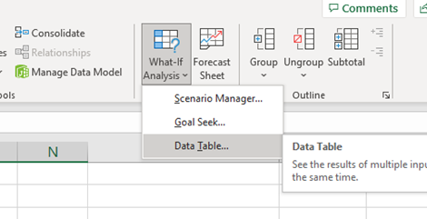
Then go to “What-If Analysis” and click on “Data Table…” (shown in Figure 10.10)
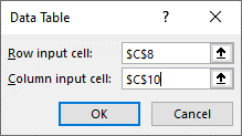
The row input in this case is the initial “Units Sold” cell and the column input is the “Variable Cost per Unit” cell. Under the “inputs” section of the spreadsheet as shown below in Figures 10.11 and 10.12.
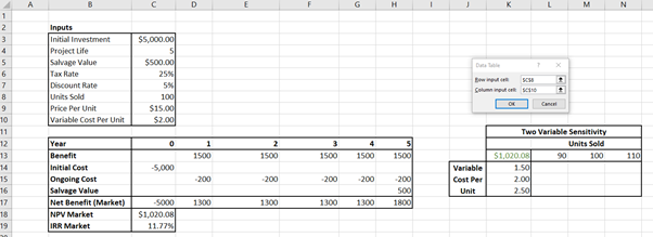
Once you click “Ok” the matrix will fill with the results of the two-factor sensitivity analysis as shown in Table 10.9 below.
See if you can replicate this table by downloading the spreadsheet here: Example10_5
Best-Worst Case Scenario
Best-worse case analysis involves identification of various combinations of inputs to generate a pessimistic and an optimistic outcome. This is then evaluated relative to the best guess scenario. For example, often in infrastructure projects best-worst case sensitivity analysis involves varying key cost inputs by -/+ 25% of their original value.
There is no golden rule on how much variation around the best guess outcome is required. However, 20-25% is fairly standard for capital heavy projects such as infrastructure developments.
Example 10.6
Consider the same company from Example 10.4 and 10.5 above. To implement the best-worst case sensitivity analysis an analyst needs to start with the point estimates (the best guess) and select the variation on either side of the key variable that is appropriate. Suppose from the information above we conduct a sensitivity analysis using the information in Table 10.10:
From this, to calculate the best-worst case results we need to calculate the relevant input values using the deviations in the costs and benefits. Note that for pessimistic outcomes decrease the values of benefits and increase the values for costs (and vice versa for optimistic estimates).
Calculating the appropriate inputs gives the results in Table 10.11 below.
From this point to find the NPV under each three scenarios, we input the values from the table above. i.e., to estimate the pessimistic outcome we change units sold to 80, the price per unit to $12, the variable cost to $2.50 and the initial investment cost to $5,500. This will give the following NPV’s and IRRs under the pessimistic, best guess and optimist scenarios.
| Best Worst Case | Pessimistic | Best Guess | Optimistic |
|---|---|---|---|
| NPV | -$1,817.83 | $1,020.08 | $4,464.13 |
| IRR | -7.16% | 11.77% | 35.08% |
Note that the results for the best guess in Table 10.12 were the same initial results using the point estimates from the initial CBA (as shown in Examples 10.4 and 10.5).
See if you can replicate this table by downloading the spreadsheet here: Example10_6
Simulations
Simulation analysis can be used as part of the sensitivity analysis. Simulations allow an analyst to test many assumptions regarding the project at the same time. When using simulation methods, we create a distribution of net benefits for each key input based on some key assumptions about the probability distribution of the underlying inputs in the CBA. Simulation analysis allows the exploration of uncertainty through the application of statistical techniques. The outcome provides the analyst with a range of statistical probabilities associated with the final outcome. Simulation will also provide insights into not only the expected value of the NPV, but the dispersion (variation) of the expected value.
One of the most popular methods for simulation in CBA is Monte Carlo simulation. Monte Carlo simulation is a computer simulation process that uses repeated random sampling. For each uncertain input, the analyst specifies a probability distribution. These distributions are drawn from once for each input, for each computation. The underlying input distribution can follow a uniform probability distribution, a continuous probability distribution, a triangular probability distribution or a cumulative probability distribution. These values drawn from the input distributions are then used to calculate the NPV. Repeating the process of drawing from the input distributions allows an analyst to estimate a distribution for the net present value which will provide in information on the expected NPV and standard deviation (along with other descriptors of the project inputs and outcomes). The standard deviation of the project to get a better understanding of potential risk.
Overall, simulation provides a structured approach to incorporating uncertainty and risk into the evaluation of the policy, program, or project under consideration.
Threshold Analysis
The final aspect we consider in this chapter is threshold analysis. Threshold analysis is an extension of sensitivity analysis used to identify a minimum or maximum value of an input within the cost-benefit analysis. Specifically, threshold analysis aims to identify a specific goal for a value under consideration to be achieved to overcome a threshold point. For example, a company may want to find a minimum NPV or a tax rate that would meet a hurdle IRR which can be determined by conducting a threshold analysis.
Example 10.7
Example – Threshold Analysis
Again, using the example from before summarised in Table 10.13 and Table 10.14 below:
Currently, the best guess NPV is $1,020.08 when the discount rate is 5%.
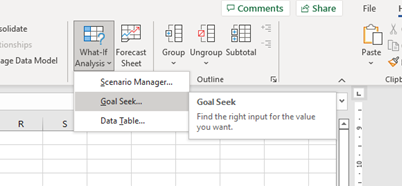
Suppose the company wishes to determine the discount rate that would achieve a minimum NPV of $1,500. To complete the threshold analysis, go to the Data ribbon. Click on the “What-If Analysis”. This time click on “Goal Seek” as shown in Figure 10.13 below:
You will see the following pop-up window:
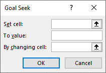
In “Set Cell”, select the cell you wish to change. In this case it would be the cell which contains the NPV of the project. In the “To value” box indicate the value you would like the input to take (in this instance $1500). The “By changing cell” should reference the cell you want to change to achieve your minimum outcome, in this case you should select the discount rate. In this example the result of inputting this information is as shown in Figure 10.15.
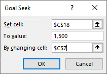
After clicking “OK” the “By changing cell” will change to the threshold value. In this instance the discount rate is changed to 2.41%. This discount rate is the minimum discount rate that would achieve the requirement for the net present value to equal $1,500.See if you can replicate this result by downloading the spreadsheet here: Example10_7
Communicating the Results
It is possible to deal with risk and uncertainty using expected value analysis and sensitivity analysis. It is important to convey the information in the sensitivity analysis clearly to the decision-maker. A good starting point is using tables and graphs. There are many graphs that can be used for a sensitivity analysis. It is common to include the NPV curve as it indicates the sensitivity to the discount rate. Bar charts, pie charts and line graphs may also be appropriate. When choosing a graph, consider what you would like to communicate to the reader of the CBA.
Revision
Summary of Learning Objectives
- When conducting a cost-benefit analysis, an analyst often relies on estimates for variables that cannot be predicted with complete accuracy. Consequently, the result of the CBA is subject to risk and uncertainty as the results cannot be determined with complete confidence. Therefore, an analyst must evaluate the risk and uncertainty associated with the evaluation of a policy or project.
- An analyst can use expected value analysis to calculate the expected NPV and the standard deviation of a project.
- We assume the decision-maker of a CBA is risk neutral. However, individuals who present their WTP may be risk averse, risk neutral or risk seeking.
- By changing the cells in an Excel spreadsheet, it is possible to implement partial sensitivity analysis (one variable and two variable analysis). It is also possible to conduct a best-worst case scenario by varying the inputs by -/+20-25% to compare the results against the best case (point estimates). Excel can also be used to implement a simulation for sensitivity analysis.
- The results of a sensitivity analysis can be communicated using tables and graphs.
- For example, an analyst suffering from optimism bias may overestimate the potential benefits of a project or underestimate the potential costs leading to the potential for an incorrect decision. ↵
- It is possible to use the coefficient of variation to determine whether a project is worth the risk i.e., calculate
 . ↵
. ↵ - As mentioned in Chapter A1, we specified “Perform a sensitivity analysis” as step 8 in the 9-step framework for conducting a CBA ↵
- For example, in the worked example from the Appendix, we used a 5%, 10% and 15% as discount rates in our estimation of the net present value. ↵
- Known as a partial sensitivity analysis. ↵
