
Chapter 5: Market and Investor Analysis
Learning Objectives
After completing this chapter, students should be able to:
-
Evaluate and create a market CBA.
-
Use incremental analysis to select between projects.
-
Compare and contrast sunk costs and working capital in project evaluation.
-
Implement loans, interest rates, depreciation, and taxes in financial appraisals.
-
Develop a CBA from the investor perspective.
Reminder: Net social benefit will be different from net private benefits if market failure exists in the project or program being evaluated. At this stage we assume that all benefits and costs can be accounted for, and market failure does not occur in the scenarios we analyse to keep concepts simplified. We will introduce market failures into our CBA analysis in Parts 3 and 4.
Market Perspective Basics
The market CBA utilises market prices to estimate the costs and benefits in financial terms to the economy. It does not correct for any market failures and ignores taxes, financing, and interest repayments. Put simply, the market perspective will account for tangible market transactions in the form of benefits and costs at market price regardless of who those benefits and costs accrue to. Usually a market analysis will include: (1) any initial investment costs to implement or start a project including working capital, (2) any salvage/horizon values and (3) any ongoing benefits and costs that accrue over the life of the project – all measured using market prices.
Example 5.1
Example: Market Analysis
Company X is a printing business. Currently the company only has traditional paper printers. Due to current demand in the market, Company X is considering purchasing a 3D printer to provide the additional service to customers. The 3D printer will cost the company $5,000 as the initial investment and will require maintenance at a cost of $350 per year over the expected life of 5 years. The expected benefit from the printer is an additional income of $1,500 per year at the current year 0 market price. At the end of the 5-year period, Company X would need to salvage the 3D printer for 10% of the initial cost. Conducting a market analysis, we would get the following table:
The status quo in this case is to not purchase the 3D printer and continue to only use the traditional printers the business currently owns. The 3D printer should only be purchased if the net present value is greater than zero. If we assume the correct discount rate for this project on behalf of Company X is 5%, the net present value of the project is $370.66. Consequently, the purchase of the printer should be undertaken.
If you would like to replicate the result for this example, please download this spreadsheet: Example5_1
The result of the market perspective is exactly what we have discussed up to this point in the course. We want to build on this foundation level understanding to further develop the CBA.
Incremental/Marginal Analysis
When considering some cost-benefit analysis projects, it is important to understand that we may want to look at the marginal gains from additional projects as part of the analysis. Consequently, incremental analysis in CBA is also sometimes referred to as marginal analysis. This method is specifically useful when a project is required to be undertaken in some form. For example, if a policymaker requires an upgrade to a traffic light road intersection. However, the government may also consider the addition of improved footpaths. To evaluate whether the additional gains from undertaking the upgrade to the footpaths and traffic lights combined, we can evaluate the incremental net benefit of the project, treating the initial investment project as the base case scenario.[1]
It is also important to note that incremental investment analysis is similar to finding the crossover rate (from Chapter 2). However, with the crossover rate, the comparison is between two different projects. When looking at the marginal analysis, the focus is on the additional investment or extension of the project under consideration.
This method of incremental analysis is often used in environmental projects and healthcare projects where interventions are required by government. The government seeks to evaluate whether the marginal gain from the additional improvements or expenditures is better than the base case project.
Example 5.2
Example: Incremental Investment.
Suppose that Company X is required to purchase at least one 3D printer as part of the terms of a contract with a customer. In this case, the base case will be the purchase of a single printer. To determine if it is worthwhile to purchase two 3D printers instead of just one, we can evaluate the incremental gain from having two printers compared to purchasing the required single printer.
Given the net benefits outlined in Table 5.2, we can calculate the incremental benefits by subtracting (1) from (2).
After calculating the incremental net benefit in (3), we can then calculate the net present value or the internal rate of return for this stream of benefits. Assuming a 5% discount rate the incremental NPV is -$62.29 and the IRR is 4.57%.
To attempt this example yourself, download the spreadsheet found here: Example5_2
When conducting incremental analysis remember that you subtract the base case scenario from the alternative that is being considered i.e., in Example 5.2 above, we subtract row 1 from row 2 as row 1 is the base case scenario. The difference is summarised in the incremental net benefit stream in row 3.
Working Capital
Working capital is inventories needed to be able to produce a good or service as part of a project. It is considered the operating liquidity of a project and captures assets, cash, accounts receivables, inventories, and materials. Usually in the case of cost-benefit analysis, we include working capital in a CBA when a project has initial inventory investment requirements. Working capital often starts in Year 1 when production of the good or service begins, and inventories are purchased. Working capital can then be increased or decreased throughout the life of the projects. At the end of the project, working capital is reversed out of the project as a benefit. Consequently, all changes in working capital must be accounted for in the costing of the project. When purchasing working capital, we treat the cashflow as a cost (negative) and when we sell working capital, we treat it as a benefit (positive).
Example 5.3
Example: Working Capital
Returning to the example of Company X from Example 5.1.
Company X requires working capital in the form of filaments for the 3D printer. In year 1, the company purchases $50 worth of filaments. In year 3, Company X decides to purchase an additional $50 worth of filaments for their inventories increasing the total working capital to $100. Working capital is then sold back at the end of the project in year 5.
Table 5.3 shows the stock of working capital over the 5-year period of the project. However, when accounting for working capital in a CBA, we only consider the changes in working capital as represented in Table 5.3. These changes in working capital are treated as an outflow when the working capital is purchased (negative) and an inflow (positive) when the project ends. Consequently, the balance of the change in working capital over the life of the project should be zero i.e. the sum of the change in working capital row must equal zero.
| Year | 0 | 1 | 2 | 3 | 4 | 5 |
|---|---|---|---|---|---|---|
| Working Capital | 50 | 50 | 100 | 100 | 0 | |
| Change in Working Capital | -50 | -50 | 100 |
Table 5.4 shows how to incorporate the change in working capital in the cost-benefit analysis, leveraging off the information from Example 5.1. The addition of working capital, the net benefit changes. Assuming a 5% discount rate, we can see that the NPV of the project has decreased slightly, taking into account the timing of the working capital investments over the life of the project.
 )
)To replicate this example, you can download this spreadsheet: Example5_3
Key Concept – Working Capital
Working capital is inventories needed to be able to produce a good or service as part of a project. Changes in working capital should be included in a cost-benefit analysis.
Sunk Costs in Cost-Benefit Analysis
Most economists are aware of the concept of sunk costs. Sunk costs are costs that have already been incurred and cannot be recovered. In general, sunk costs are excluded from any future decision-making – as we cannot go back in time and change the past. Decision-making is focused on choices related to current and future projects or policies. Consequently, in CBA we exclude any sunk costs that were incurred before the evaluation of the project as these costs are irrelevant to any future decisions.
Furthermore, sunk costs are not included in CBA as there is no opportunity cost involved. By including sunk costs in the evaluation of a project or policy in CBA, we require a much higher return on the project to counteract the increased costs. Only present and future costs or benefits are assessed in a CBA framework.[2]
For example, suppose a government had already purchased some unused land for $10 million, 10 years ago. When considering using the land in the present year for a project, the government would not include the $10 million cost of the past purchase of the land. Only the opportunity cost of the land would be accounted for in the CBA.
Private Firm (Investor) Perspective
When conducting a CBA from a private perspective we are considering the project or policy from the point of view of the investor who will implement it. Therefore, the investor can be a private firm (private sector) or the government (public sector). To evaluate a project from the perspective of the investor, we are evaluating the profitability of the project – a form of financial appraisal.[3] Consequently, we need to account for loans (principal and interest), taxes, and depreciation. The way we deal with these issues is highlighted in the examples that follow.
Debt Financing
Note: Remember that the rate of interest paid on a loan is not the same as the discount rate in cost-benefit analysis. The interest rate paid on loans is often referred to as the cost of capital or cost of borrowing.
Loan repayments only matter from the perspective of private firms or investors! It is not appropriate for any debt financing to be accounted for in a social cost-benefit analysis perspective. In addition to this, we do not treat the implementation of the loan as a “cost” to the project. We include it as a separate cashflow component in the project. However, to have a full understanding of CBA it is important we understand financial appraisal basics, including why investors may take out loans for projects.
Financing has two components: (1) the principal of which is the amount borrowed from the bank or lender, and (2) the interest is the cost charged by the bank or lender to you to borrow this money. This is important for us to note as interest on debt is tax deductible which will be relevant for determining after tax profits.
To implement loans in a CBA, there are two methods in our spreadsheet. The preferred approach depends on the goal of the analysis.
(1) Method 1 implements the loan from the view of the private firm (the borrower), where the loan is treated as an inflow to the investor (positive) and all repayments are an outflow (negative).
(2) Method 2 implements the loan from the bank perspective. When implementing the loan from the perspective of the bank, the loan is treated as an outflow to the investor (negative) and all repayments are an inflow. This method is preferred if you want to calculate the internal rate of return on debt.
The remaining net benefit after accounting for loan repayments is the “net private benefit” or equity on investment. Equity is the gain to the private investor. Consequently, the goal of the investor perspective is to determine the return to the private firm via the equity received from the project.
Implementing Debt Financing in Excel
The functions to implement the loans in Excel are outlined in Example 5.4 below. Note the following information on the Excel functions used for loans:
=PMT() function calculates the annuity of the loan – i.e., This function calculates the payment for a loan based on constant payments and a constant interest rate for the life of the loan (i.e., an annuity repayment). This value is the same for all periods accounted for in the project. The repayments can be yearly, quarterly, monthly, etc.
=PPMT() function calculates the amount of principal that contributes to the loan repayment assuming the loan is paid as an equal annuity for the life of the loan.
=IPMT() function calculates the amount of interest that contributes to the loan repayment assuming the loan is paid as an equal annuity for the life of the loan.
Example 5.4
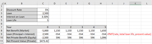
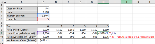
Following from Example 5.1. Assume that Company X requires a loan for the 3D printer worth $2,500 at a 3.5% cost of borrowing and the appropriate discount rate is 5%. Starting with the Net Benefit from the market analysis (the last row of Table 5.1), it is possible to incorporate the loan using either of the following two approaches as shown below:
Approach (1) – borrower’s view of debt
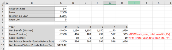
In this instance we treat the initial loan as a positive inflow and the repayments as a negative outflow. Calculating the interest on the loan will give the following:
To implement this in Excel, use the =PMT() function to calculate the principal and interest for row 9 as shown in Figures 5.1 and 5.2. Note that the repayments on the loan are equal in size to the value of $554. This is because the loan is being paid back per year in equal instalments (an annuity).
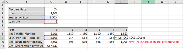
As the loan uses the same formula you can lock the formula cells using the F4 button in windows (on Mac use function + command + T) as shown in Figure 5.3 below. The “$” in front of the letters locks the column and the “$” in front of the number locks the row. This way you can copy the formula across for all years in the project. Remember to only lock cells where appropriate.
Approach (2) – bank/lender view of debt
In the instance where we approach the loan from the perspective of the lender we still use the =PMT() function to calculate the principal and interest for row 9 as shown in Figures 5.1 and 5.2, however we just invert the signs with a negative “-“ in front of the =PMT(). This is highlighted in purple in Figure 5.4 below.
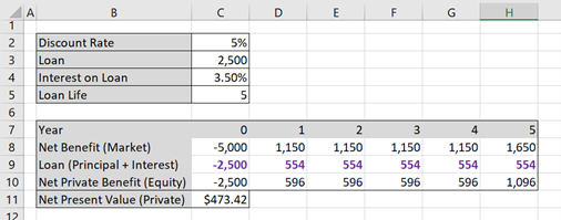
In both Approach (1) and Approach (2) we achieved the same Net Private Benefit. In addition to this it is clear that the Net Benefit on the Market is equal to the Debt Financing and Net Private Benefit. i.e. row 9 and 10 sum to row 8 in the analysis.
To replicate this result, you can download the spreadsheet here: Example5_4
It is also worthwhile to note that the total loan repayment is equal to the sum of the principal and interest payments (PPMT and IPMT solutions sum to the PMT solution). This makes it easier to check you have implemented the functions correctly in Excel. Take caution with negative and positive numbers in the cells for this analysis – think of the logic related to how we will need to deal with interest payments as a tax deduction as this will be important later for determining after tax profit (see this section on interest, depreciation, and taxes liable).
One important thing to note is that often it is useful to separate out the principal and interest repayments on a loan. This is because for an investor the interest repayment can be subtracted from the before tax profits. An illustration of how to separate these out is show in Example 5.5 below.
Example 5.5
Example: Separating Principal and Interest
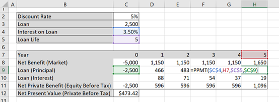
Following from the Example above, separating the principal and interest is easy. In Excel =PPMT() function will calculate the principal and the =IPMT() function will calculate the interest. Figure 5.5 and 5.6 demonstrate an example.
Note that the “year” component should not be cell locked as it should vary over the life of the loan. i.e. in year 1 =PPMT($C$4,D7,$C$5,$C$9) and in year 5 =PPMT($C$4,H7,$C$5,$C$9). More specifically, the red cell in the figure below will move between years 1-5. The remaining cells are constant values from the variable section of the spreadsheet. This way you can drag your formula across.
The =IPMT() function follows the same process as the PPMT function. To check if you have completed it correctly, you can add the principal (=PPMT) and interest (=IMPT) together and it should equate to the annuity of the loan found using the =PMT function.
To replicate this result, you can download the spreadsheet here: Example5_5
Example 5.5 also illustrates the relationship between the principal and the interest. Specifically, interest is charged based on the remaining balance of the loan. As each repayment is made, the balance of the loan decreases and consequently, the proportion of principal repaid in each subsequent repayment increases. This is observed by the increasing values of the principal component and decreasing values of the interest component on the loan. However, if you add the principal and interest in each column, it will equate to the total annuity found by using the =PMT() function.
Debt Financing, Gearing and the IRR on Equity
As illustrated in Example 5.4, we observe the following result:
(1) 
Comparing the NPV’s for Example 5.1 and Example 5.4 we can see that the NPV on the market is $370.66 and the NPV for the Printing Company X (the private investor) is $473.42. From the private investor perspective, the loan improves the profitability of the project. This begs the question – why not just take out many loans for all projects?
To understand this more effectively it is a good idea to investigate the internal rate of return on debt and equity. However, it is important to note that the internal rate of return on equity is not the difference between of the IRR on debt and the IRR on the market (i.e.  ). To calculate the IRR on equity we need to take into account the proportion of debt and equity involved in the project. i.e., the debt-equity ratio. We then input these percentages into the following formula:
(2) 
Example 5.6
Example: Debt to Equity Ratio and Gearing
To calculate the IRR on Equity, we can calculate the IRR on the market and on the debt by using the IRR formula. To illustrate this, we can use Example 5.4. Again we assume a 5% discount rate.
Firstly, we want to calculate the IRR on debt, we must use Approach (2) for the loan to find the IRR. Otherwise, you will calculate the incorrect IRR as IRR as a function in Excel requires an outflow as the first cell in the function, followed by inflows and /or outflows i.e. the first cell must be negative when using the =IRR() function. Calculating the IRR for the market and the IRR on debt using the =IRR() function in Excel, as demonstrated in Figure 5.7.
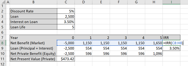
The result of this calculation is provided in Table 5.6 below:
Once we have the IRR for the Market (7.51%) and the IRR on Debt (3.50%). As observed in this example, the debt-to-equity ratio is 50:50. There is a loan worth $2,500 and the remainder of the investment in capital stock is Company X’s equity of $2,500. We can apply the formula from equation (2).

As can be seen from the example the IRR on Market  IRR Debt + IRR Equity.
To replicate this example you can download this spreadsheet: Example5_6
As can be seen from the example the IRR on Market IRR Debt + IRR Equity. Changing the ratio of debt-to-equity will change the result of the internal rate of return on equity and therefore the profitability of the project to the investor. In fact, as the proportion of debt increases, the IRR on equity will increase. For example, if we have a market IRR of 8% and IRR on debt of 5%, if the debt-equity ratio is 50:50, then the IRR on equity would be 11%. If the IRRs for the market and debt remained the same but the debt-to-equity ratio increased to 80:20, then the IRR on equity would be 20%.
From this example we can see that it is better for a company to take out a loan when investing in a project. However, we should note that if the debt-to-equity ratio is too large it would be unlikely to find a bank to lend money as banks will not lend to projects with very high levels of debt. Banks do not lend at high debt-to-equity ratios as it would be considered risky.
The IRR on equity is important. However, it should not be the driver of the decision in CBA as it does not capture the social aspects of cost-benefit analysis. Additionally, the IRR on equity can make a good project look like a bad investment and a bad project look like a good investment. This highlights the role of gearing in CBA – IRR is misleading as a measure of net benefits.
Depreciation and Tax Liability
Depreciation and taxation laws vary from country to country. This section provides a basic approach to dealing with depreciation in the context of an investor perspective. It is important if you are applying these concepts in the real world to consult the relevant taxation services.
The initial investment cost for an asset captures the value of the investment. Including depreciation in a CBA as a cost would result in double counting the value of the initial investment. This is because depreciation is already accounted for in the initial investment, so adding it again as a cost would mean counting it twice. Consequently, depreciation is not included in the market, social or disaggregated cost-benefit analyses.
However, depreciation in the financial appraisal space is essential as a bookkeeping mechanism. Including depreciation in the evaluation of the investor perspective amounts to setting aside part of the project’s income to finance equivalent capital expenditure in the future. This is a useful approach to project evaluation when you are expecting to replace large amounts of equipment or capital when rolling projects over. Additionally, from a private perspective we may need to consider depreciation in relation to profits as part of the calculation of taxable income. In this instance we can treat depreciation as an outflow that reduces taxable income.
Key Concept – Depreciation in Investor CBA
Depreciation is about spreading the cost of an asset over its useful life and matching expenses with revenue. It is a financial mechanism and therefore should only be accounted for in the investor CBA. Always use straight line depreciation.
Depreciation should never be used in the market or social perspectives.
When calculating depreciation in CBA, the straight-line method is used. To keep it simple when using straight line depreciation, we take the value of the asset and divide it by the asset’s useful life.[4] Depreciation is then subtracted from the firms before tax profits. Specifically, we calculate this in two steps:
(1)  ,
,
then calculate
(2) 
Example 5.7
Returning to Example 5.1, Company X is considering purchasing a 3D printer to provide the additional service to customers. The 3D printer will cost the company $5,000 as the initial investment and will require maintenance at a cost of $350 per year over the expected life of 5 years. The expected benefit from the printer is an additional income of $1,500 per year at the current year 0 market price. At the end of the 5-year period, Company X would need to salvage the 3D printer for 10% of the initial cost. Assume a 5% discount rate.
Assuming straight line depreciation, and a 25% tax rate – the private perspective can be calculated by taking the market perspective, subtracting the taxes paid on profits. Taxes paid on profits must take into account depreciation and interest paid on loans. In this case we have assumed there is no loan and only depreciation needs to be accounted for. The straight-line depreciation value would be:

To calculate before tax profits for each year we take the revenue (1,500) and subtract the ongoing operating cost (350), and the depreciation (1,000). This leave a before tax profit of $150 as shown in Table 5.7. With a 25% tax rate, the tax liable is $37.50. Note that taxes can be inputted as a negative value or a positive value in Excel. But to find the after tax for each year the taxes are subtracted from the Net Benefit (Market).
To replicate this example, you can download the spreadsheet found here: Example5_7
Combining Debt Financing & Depreciation in the Investor Perspective
The last stage of the investor perspective is to combine all elements discussed in this chapter. i.e., calculate the market perspective including debt financing and depreciation. Both interest and depreciation can be subtracted from the investors profit before calculating the tax liable. This is illustrated in Example 5.8 below.
Example 5.8
Example: Including Both Debt Financing and Depreciation
Assume we are considering Company X’s options to take a loan and depreciate the new 3D printer. The 3D printer will cost the company $5,000 as the initial investment and will require maintenance at a cost of $350 per year over the expected life of 5 years. The expected benefit from the printer is an additional income of $1,500 per year at the current year 0 market price. At the end of the 5-year period, Company X would need to salvage the 3D printer for 10% of the initial cost.
In addition to this, Company X would like to take a loan worth $2,500 to help finance the project. The interest rate on the loan will be 3.5% and the loan life will be equivalent to the life of the project (5 years). Company X would also depreciate the 3D printer over the 5 years using straight line depreciation.
We have the following information in Table 5.8:
| Discount Rate | 5% | Benefit | 1,500 | |
|---|---|---|---|---|
| Loan | 2,500 | Initial Cost | 5,000 | |
| Interest on Loan | 3.50% | Ongoing Cost | 350 | |
| Loan Life | 5 | Salvage | 10% | |
| Tax | 25% |
Step 1 is to calculate the market perspective first using the annual benefit, initial cost, ongoing cost and salvage value as shown in part (a) in Table 5.9 below.
Step 2 is to calculate the Net Private Benefit after loan repayments in part (b) of the table. Note that we have separated out the principal and interest to make it easier to account for the interest.
Step 3 is to calculate the before tax profit by subtracting operating costs, depreciation, and interest repayments from the revenue (shown in part (c)). We then multiply this profit by the tax rate in the last row of part (c).
Finally, taking the difference between the Net Private Benefit and the taxes liable will provide the equity to the firm. Once this is found, we can apply the =NPV() function in Excel to find the NPV to the private investor, in this case Company X.
As can be seen, after accounting for salvage, depreciation, debt financing, and taxes liable the NPV of the project is positive. Therefore, Company X should undertake this project and purchase the 3D printer using a financing option.
To replicate this example, you can download the spreadsheet found here: Example5_8
Timing of Debt Repayments
When we covered compounding in Chapter 2 we assumed that each period was compounded yearly. However, it is important to note that for debt financing interest may be compounded daily, monthly, quarterly, or yearly depending on the terms agreed to by the bank. Based on this, adjustments may need to be made to the interest rates used to ensure that the interest rate appropriately reflects the timing of benefits and costs.
Effective Annual Interest Rates
Some loans have a monthly rate and need to be converted to annual rates. To do this we can calculate the effective annual interest rate, and subsequently use the effective annual interest rate in the analysis. To calculate the effective annual interest rate, we use the following formula:
(3) 
where:
 = Effective Annual Interest Rate.
 = interest rate (this can be daily, bi-annually, quarterly, monthly etc.)
 = number of compounding periods in a year based on the interest rate period.
The equation above indicates that the effective annual interest rate will always be higher than the stated rate if there is more than one compounding period. This is illustrated in Example 5.9 below. Additionally, all things held constant – the more compounding periods the higher the EAR.
Example 5.9
Example: Comparing Interest Rates
Suppose a company is considering a loan. There are two options under consideration and the firm would like to identify which one to select.
- (a) interest rate is 14% compounded quarterly.
- (b) interest rate of 15% compounded annually.
To compare the two interest rates, we need to convert option (a) to an equivalent annual interest rate as follows:

Comparing the options, option (a) has an annual interest rate of 14.75% and option (b) has an annual rate of 15%. Consequently, the firm should select option (a) as it has the lower yearly interest rate.
If a policy or project has a compounding period that is not annual but has an annualised interest rate, the effective annual interest rate would need to be converted rate to match the appropriate timeline (for example, daily, monthly or quarterly etc.). For example, you may take out a loan over 10 years with an annual interest rate, however the repayments may be monthly. In this case you can rearrange the formula for the effective annual rate and solve for () which is the monthly interest rate i.e., we would use the formula  where is the interest rate, EAR is the effective annual interest rate, n is the number of periods for compounding. This is used more often in financial appraisals compared to social cost-benefit analysis. Once we have the appropriate interest rate that matches the compounding periods, we can use it to determine the correct loan cost to an investor.
Compound Interest – For Loans
In some instances, a private firm may wish to calculate the total amount that will be paid on a loan. To do this we can apply the following formula:
(4) 
where
 = the amount of the loan paid
 = principal of the loan
 = the duration of the loan
= interest rate
= number of times interest applied per time period
This is not often used for cost-benefit analysis specifically, but the compounding formula is useful in some instances of evaluating projects from a financial approach.
One Final Note.
This chapter considered the market and investor perspectives for cost-benefit analysis. The market perspective used market prices to evaluate a project with the consideration of fixed investment costs, salvage/horizon values and working capital. The investor or private perspective build on the market analysis as private firms pay market prices to implement a project or program. In the investor perspective, we calculated profits considering debt financing, depreciation, and taxable income. The remainder of the net benefits after this is completed is the net benefit to the private investor.
To round of this chapter, we briefly discuss how a market and private analysis would capture interest from investment and direct government subsidies as benefit inflows, where appropriate. These are more complicated to implement, but the basic processes are the same as demonstrated above. Interest from investments would be positive and would therefore need to have taxes paid on interest income. Direct subsidies can be treated as an additional benefit in the private analysis. A firm would not pay taxes on subsidy income (as this would be counterintuitive to the subsidy). Indirect subsidies will be covered later in the analysis.
In later chapters we will cover the social cost-benefit analysis perspective, and the distributional impacts of the social CBA. The goal of this book is to implement social CBA that evaluates potential policies, projects, and programs from the social perspective. This chapter covered important concepts that allow an analyst to identify the incentives of the investor via a market price approach. However, we still need to deal with market failures. Before we can do this, we need to revisit some important microeconomic concepts in Chapter 6, 7 and 8.
Revision
Summary of Learning Objectives
- A market CBA perspective uses cash inflows and outflows at market prices. We need to capture any salvage values and working capital changes in the market perspective.
- The incremental analysis allows for a comparison between a base case project that is required and additional combinations of that project (relative to the base case).
- Sunk costs are excluded from CBA. Only changes in working capital are accounted for in CBA.
- Debt financing and depreciation are only considered in the investor perspective as the investor perspective is equivalent to a financial appraisal of a project.
- We can evaluate a project or program from the investor perspective. The debt-to-equity ratio impacts the IRR to the private investor.
- There is no status quo comparison when using incremental analysis, we compare against the base case scenario. ↵
- For ex-ante CBA. However, ex-post CBA should also exclude any sunk costs that occurred before the start of a project. ↵
- This is often considered necessary if we wish to identify the distributional social impacts of a project. This analysis allows for the identification of the benefits that directly accrue to an investor. The remaining benefits and costs can then be identified and allocated to the various stakeholders with standing in the project. ↵
- Depending on the context and standards of relevant department or companies it may be necessary to subtract the salvage value from the value of the asset might be required when taking a financial analysis approach. In CBA we often do not incorporate this method in the instance the salvage value may be negative instead of positive. By taking the approach of salvage + full depreciation we end with a more conservative estimate of the NPV. ↵
